1. Introduction

The variation in the position of sun in the sky is a natural phenomenon that can be observed on daily basis. The phenomenon has served for the consideration of an approximate measure of local time [1]. The solar trajectory as observed on the earth surface is a result of the combined effects of the rotation of earth along its axis and the revolution of earth around sun.

As the rotation axis of the earth is tilted at a certain angle to the plane of the earth's orbit around the sun, and the revolution of the earth around the sun follows an eccentric elliptical path, the solar trajectory calculation is not that trivial. The trajectory of the sun as observed at a specific location on a specific time of the day (for all days) of a year, is called the analemma. The difficulty in practically observing this phenomenon is that it requires a whole year to collect the data [2]. The structure of an analemma looks similar to that of the number "8". But unlike the number "8", the two loops of the analemma are unequal in size with one of them larger than the other. In astronomy, the analemma is considered one of the most difficult and demanding phenomena to imagine because it is never present all at once. It requires a virtual image made with the solar position data collected at the same time of day, for several days, throughout the year [2].

Modelling the analemma requires the ability to determine the position of the sun in the sky at a given time, date, and location. Another challenge lies in accurately representing the analemma's shape in a way that is easily understandable to viewers, particularly those unfamiliar with the cartographic and astronomical projection techniques used by geographers and astronomers [3]. In this paper an attempt has been made to bridge this gap so that the common people, science students and the professional engineers could make use of this information for solar insolation and atmospheric temperature calculations.

The solar position algorithms are sophisticated schemes commonly used to compute the position of the Sun in ecliptic, celestial and horizontal coordinates. On the internet it is also possible to find some computer codes to calculate the position of the Sun in the sky [4]. The purpose of this paper and the companion papers [5, 6] is to present and elaborate a self-contained material suitable for scientists, engineers and common people to be able to determine and interpret the solar position in the sky. In our earlier papers [5, 6], the methodologies for calculation of the solar elevation angle, the solar azimuth angle and the Equation of Time were presented. In this paper, after this Introduction Section 1, the Section 2 presents the position of the sun in the sky, as observed from the earth. Section 3 presents the solar trajectory plots and the solar analemmas for some selected cities, for demonstration purpose, only. The results are discussed in Section 4, followed by conclusions in the Section 5.

2. Solar Position in the Sky

It can be observed easily, that the sun is not at the same position in the sky, at the same clock time, every day along the year. The reason is that the clock time is based on the consideration of a fictitious earth that rotates around the sun in a circular trajectory with constant tangential/angular velocities [7, 8]. Additionally, it is also assumed in the measure of clock time, that the sun is always located at the equator of earth.

On the other hand, we know that the trajectory of the earth is elliptical, and its tangential velocity, $v_t$ as well as the solar position relative to the equator of earth (the declination angle, $\beta$), both are varied in time all along the year. The difference between the clock time and the position of sun in the sky (called the solar time), is known as the correction of time, or simply, the equation of time [6].

It may be recalled [6], that the solar zenith angle is calculated by the following equation:

and the solar elevation angle can be obtained by subtracting the solar zenith angle from 90°. Similarly, the solar azimuthal angle is calculated by:

where $\rho$ is Earth's rotation angle $0\le \rho \le 2\pi$, $\beta$ is the declination angle between the Earth's equator and the vector from the Earth to the Sun (it oscillates from $-{23.45}^{\circ }$ to ${23.45}^{\circ }$), and $\delta$ is the latitude on the Earth's surface where the observer is located.

Figure 1 Map of the solar azimuth angle is measured from north of the observer's horizon plane ${\alpha }_a$ and the solar elevation angle ${\alpha }_e$. The observer is located at a latitude $\delta ={19.4}^{\circ }$. Four days along the year 2013 are shown. The sunrise and the sunset regions are displayed on either side of the graph. The declination angle $\beta$ at the beginning of the day in degrees (Declin. start) and the declination angle $\beta$ at the end of the day in degrees (Declin. end) are also displayed. The legend "Sun is north" (on June 21) means that the declination angle, $\beta$, is higher than the latitude, $\delta ={19.4}^{\circ }$, of the place (Mexico City).

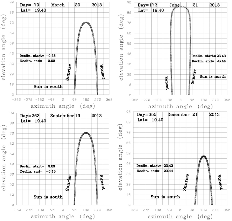
Figure 1 presents for four days (March 20, June 21, September 19 and December 21) of the year 2013, a two-dimensional map, in which the solar azimuth angle ${\alpha }_a$ is the abscissa and the solar elevation angle ${\alpha }_e$ is the ordinate, corresponding to a latitude $\delta ={19.4}^{\circ }$ (for Mexico City). The angles ${\alpha }_a$ and ${\alpha }_e$ are calculated using the declination angle ($\beta$). The declination angle ($\beta$) at the beginning of the day and at the end of the day (see the values of Declin. start and Declin. end), as well as the sunrise and sunset regions, are displayed in each panel. It can be observed in Figure 1 that on some dates of the year, the Sun is north of the place, hence the physical interpretation of the angles ${\alpha }_e$ and ${\alpha }_a$ is different. That is, when the Sun is north of the place, the solar azimuth angle is measured from north of the observer's horizon plane in the interval . Where, the interval from ${90}^{\circ }$ to $0^{\circ }$ corresponds to the region from sunrise to noon, while the interval from $0^{\circ }$ to $-{90}^{\circ }$ corresponds to the region from noon to sunset. Then when the Sun is north of the place under consideration: (i) at noon ${\alpha }_a=0^{\circ }$, and (ii) as the Sun is north of the observer's horizon plane, the elevation angle ${\alpha }_e$ is measured from north of this plane. Similar calculations were also performed for the Holy City of Mecca and Islamabad, and the data was used in the presentation of analemmas for these cities (see Section 3).

It was shown in our previous paper [6] that, in a fixed coordinate system, the position vector of the Earth, ${𝐱}_E\left(t\right)$, the position of an observer, ${𝐱}_{\text{obs}}\left(t\right)$, and the vector, ${𝐱}_{E\text{–obs}}$, which is the relative vector from the center of the fictitious Earth to the observer (that is ${𝐱}_{E\text{–obs}}\left(t\right)={𝐱}_{\text{obs}}\left(t\right)-{𝐱}_E\left(t\right)$), are as below:

In the case of the true Earth, which moves in an elliptical trajectory, it has an angular velocity $\left({\Omega }_{\text{Ell}}\left(t\right)=\frac{d\theta \left(t\right)}{dt}\right)$, which is not constant over time and position. In our earlier papers [5, 6], by making use of two Cartesian coordinate systems, one with origin at the focus of the ellipse (at the solar position), and the other with origin at the center of the Earth (moving in an elliptical orbit), we derived a relation like that for a true Earth.

Figure 2 Circular trajectory of the fictitious Earth. Vectors ${𝐱}_E\left(t\right)$, ${𝐱}_{\text{obs}}\left(t\right)$ and ${𝐱}_{E\text{–obs}}\left(t\right)$ for three selected days. Top row: 1st day, middle row: 17th day, and bottom row: 99th day. At noon or initial time (first column, from left) and after 24 hours or 1440 minutes (fourth column, from left) the three vectors are collinear. Second column (from left): after 432.09 minutes (0.3 of the day) from noon. Third column (from left): after 1296.2 minutes (0.9 of the day) from noon. The time, $t$, is given in minutes and days. The angle ${\omega }_{\text{circ}}t$ is given in degrees, while the angle ${\Omega }_{\text{circ}}t$ is given in degrees.

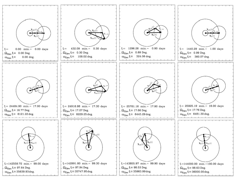
A graphical representation of the position vectors, ${𝐱}_E\left(t\right)$, ${𝐱}_{\text{obs}}\left(t\right)$ and ${𝐱}_{E\text{–obs}}$, calculated by equations (3)–(6) is shown in Figure 2, which illustrates the three selected days (top row: 1st day, middle row: 17th day and bottom row: 99th day) the vectors, ${𝐱}_E\left(t\right)$, ${𝐱}_{\text{obs}}\left(t\right)$ and ${𝐱}_{E\text{–obs}}\left(t\right)$. It is observed that at noon or initial time (first column) and after 24 hours or 1440 minutes (fourth column) the three vectors are collinear, i.e., the Sun is at the observer's zenith. Panels in the second and third columns show the three vectors after 432.09 minutes (0.3 of the day) and after 1296.2 minutes (0.9 of the day) from noon or initial time (see first column) respectively. Note that for each of the selected days, the difference between the angles ${\omega }_{\text{circ}}t$, shown in the second, third and fourth columns, and the angle ${\omega }_{\text{circ}}t$ at noon (see first column) is the same—108.02 degrees, 324.06 degrees and 360 degrees respectively. This confirms the fact that, in the fictitious Earth model, an observer sees the Sun at the same position, at the same hour of the day (for the whole year).

In order to understand the effect of the difference (at a certain time t) between the angle spanned by the fictitious Earth moves along its circular trajectory with constant angular velocity ${\Omega }_{\text{circ}}$, and the angle $\theta \left(t\right)$ spanned by the true Earth along its elliptical path with an angular velocity ${\Omega }_{\text{Ell}}\left(t\right)$ (which on some dates of the year is higher and on other dates is lower than the constant angular velocity of the fictitious Earth, ${\Omega }_{\text{circ}}$), the following scenario is formulated: Let us assume that there exists an imaginary Earth that travels with constant angular velocity ${\Omega }_{\text{Ell}}$ along an elliptical trajectory with eccentricity $\epsilon =0.1$. The angular velocity ${\Omega }_{\text{Ell}}$ of the imaginary Earth for this exercise is given as:

Then, the constant angular velocity ${\Omega }_{\text{Ell}}$ of the imaginary Earth is obtained by considering that it travels along the whole ellipse (360 degrees) in 10 days. That is, ${\Omega }_{\text{Ell}}=0.025$ Degrees/minute, which is much higher than the fictitious Earth angular velocity, ${\Omega }_{\text{circ}}=0.0006849315$ Degrees/minute (see Eq. (3)). Note that the $\theta \left(t\right)$ angle spanned by the imaginary Earth is given as $\theta \left(t\right)={\Omega }_{\text{Ell}}t$. The first component of the Equation of Time is obtained if it is assumed that: (i) the imaginary Earth travels along the elliptical path with a constant angular velocity ${\Omega }_{\text{Ell}}$; (ii) the moving coordinate system $(0,x_1,x_2)$ does not rotate as $\dot{\theta }\left(t\right)={\Omega }_{\text{Ell}}$, but as ${\Omega }_{\text{circ}}$ (the angular velocity of the fictitious Earth); (iii) the radius of the fictitious Earth $r_f$ and the radius of the true Earth $r_t$ are unitary, hence we can interchange them in the expressions. Then, the position vector of the observer, ${𝐱}_{\text{obs}}$, is modified as:

Figure 3 An imaginary scenario. Circular trajectory of the fictitious Earth (left column), and elliptical trajectory of an imaginary Earth (middle and right columns). The eccentricity of the ellipse is $\epsilon =0.1$. Vectors ${𝐱}_E\left(t\right)$, ${𝐱}_{\text{obs}}\left(t\right)$, and ${𝐱}_{E\text{–obs}}\left(t\right)$ for two selected days are shown. Top row: initial position ($t=0$ minutes), the Sun is at the zenith of two observers. Left column for the fictitious Earth, right column for the imaginary Earth. Middle row: left column after 1440 minutes (24 hours) in the fictitious Earth, Sun is at the zenith. Middle column after 1440 minutes in the imaginary Earth, the Sun is not at the zenith. Right column after 1595.84 minutes (1.108 days) in the imaginary Earth, Sun is at the zenith. Bottom row: left column after 5761.1 minutes (4 days) in the fictitious Earth, Sun is at the zenith. Middle column after 5761.1 minutes in the imaginary Earth, the Sun is not at the zenith. Right column after 6380.48 minutes (4.43 days) in the imaginary Earth, Sun is at the zenith.

Figure 4 Analemmas for Mexico City located at the latitude $\delta ={19.4}^{\circ }$. The solar azimuth angle measured from north, ${\alpha }_a$ (degrees), is used as the abscissa, and the solar elevation angle, ${\alpha }_e$ (degrees), as the ordinate. Left panel: Analemma at 10:00 A.M. Middle panel: Analemma at noon. Right panel: Analemma at 4:00 P.M.

Figure 5 Analemmas for Islamabad, located at the latitude $\delta ={33.74}^{\circ }$. The solar azimuth angle measured from north, ${\alpha }_a$ (degrees), is used as the abscissa, and the solar elevation angle, ${\alpha }_e$ (degrees), as the ordinate. Left panel: Analemma at 10:00 A.M. Middle panel: Analemma at noon. Right panel: Analemma at 4:00 P.M.

Figure 6 Analemmas for the holy city of Mecca in Saudi Arabia, located at the latitude $\delta ={21.42}^{\circ }$. The solar azimuth angle measured from north, ${\alpha }_a$ (degrees), is used as the abscissa, and the solar elevation angle, ${\alpha }_e$ (degrees), as the ordinate. Left panel: Analemma at 10:00 A.M. Middle panel: Analemma at noon. Right panel: Analemma at 4:00 P.M.

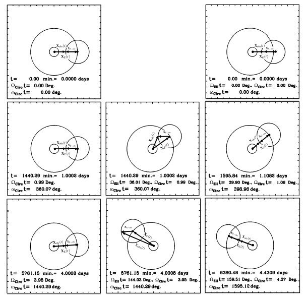
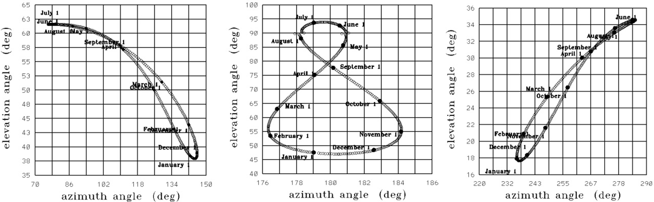
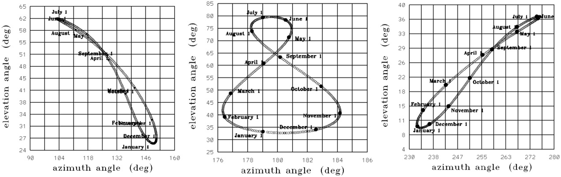
Figure 3 shows (see the middle and right columns) for two selected days, the three vectors: ${𝐱}_E\left(t\right)$, ${𝐱}_{\text{obs}}\left(t\right)$ and ${𝐱}_{E\text{–obs}}$, referred to the fixed coordinate system whose origin is located at the focus of the ellipse (at the solar position). Left column of the Figure 3 shows the results for the fictitious Earth. Top row shows that at the initial time, $t=0$ minutes, in the fictitious Earth and in the imaginary Earth, the Sun is at the zenith of the two observers. In the middle row, left column, it is shown that when the fictitious Earth has spanned ${\Omega }_{\text{circ}}t=0.9863$ degrees (i.e., after $t=1440.2$ minutes or 24 hours), the Sun is again at the zenith of the observer. However, in the middle column, it is observed that in the imaginary Earth, with elliptical trajectory, the Sun is not yet at the zenith of the observer—that is, the Sun is delayed and it is at the east of the observer. In the right column (middle row), it is observed that after $t=1595.8$ minutes (or 1.108 days), the Sun is at the zenith of the observer located on the imaginary Earth. If the elapsed time is calculated since the Sun is at the zenith of the observer on the fictitious Earth (see left column, $t\approx 1440.29$ minutes) until the Sun is at the zenith of the observer on the imaginary Earth (see right column, $t\approx 1595.84$ minutes), we obtain $\Delta t\approx 1440.29-1595.84\approx -55.55$ minutes.

A similar value is obtained from Figure 3, middle row, right column, in which the angles spanned by the two Earths along their orbits are written. That is, $\theta \left(t\right)={\Omega }_{\text{Ell}}t\approx {39.9}^{\circ }$ and ${\Omega }_{\text{circ}}t\approx {1.09}^{\circ }$. The difference between these two angles, ${\Omega }_{\text{circ}}t-\theta \left(t\right)=-{38.81}^{\circ }$. If this value is divided by the angular velocity of the Earth about its rotation axis, we obtain: $\frac{{\Omega }_{\text{circ}}t-\theta \left(t\right)}{{\omega }_{\text{circ}}}=\frac{-{38.81}^{\circ }}{0.25\text{degrees/minute}}\approx -155.24\text{minutes}.$ Note that this is the way to calculate the first component of the Equation of Time due to the eccentricity of the trajectory of Earth.

In the bottom row, left column of Figure 3, it is shown that after $t=5761.15$ minutes (or four days), the Sun is at the zenith of the observer located on the fictitious Earth. However, in the middle column (for the imaginary Earth), it is noted that after the same time, $t=5761.15$ minutes, the Sun is not at the zenith—hence it is delayed and is at the east of the observer. Note that on the right column of the bottom row, after $t=6380.48$ minutes, the Sun is at the zenith of the observer located on the imaginary Earth. From this, it is possible to calculate the elapsed time, since the Sun is at the zenith of the observer on the fictitious Earth (see left column, $t=5761.15$ minutes) until the Sun is at the zenith of the observer on the imaginary Earth (see right column, $t=6380.48$ minutes), we obtain: $\Delta t\approx 5761.1-6380.4\approx -619.3\text{minutes}.$

A similar value is obtained from the bottom row, right column, in which the angles spanned by the two Earths along their orbits are written. That is, $\theta \left(t\right)={\Omega }_{\text{Ell}}t={159.5}^{\circ }$ and ${\Omega }_{\text{circ}}t={4.3}^{\circ }$. The difference between these two angles is ${\Omega }_{\text{circ}}t-\theta \left(t\right)=-{155.2}^{\circ }$. If this value is divided by the angular velocity of Earth about its rotation axis, we obtain: $\frac{{\Omega }_{\text{circ}}t-\theta \left(t\right)}{{\omega }_{\text{circ}}}=\frac{-{155.0}^{\circ }}{0.25\text{degrees/minute}}\approx -620.0\text{minutes}.$ The results obtained in this imaginary exercise allow us to conclude that when the angular velocity ${\Omega }_{\text{Ell}}$ of the true Earth is higher than the constant angular velocity ${\Omega }_{\text{circ}}$ of the fictitious Earth, the Sun is delayed—hence it will be at the east of the observer. On the other hand, it is possible to demonstrate through a similar imaginary scenery that when the angular velocity ${\Omega }_{\text{Ell}}$ of the true Earth is smaller than the constant angular velocity ${\Omega }_{\text{circ}}$ of the fictitious Earth, the Sun being ahead of the observer will be at the west of the observer.

3. Solar Analemmas for Some Selected Cities

An analemma is a diagram showing the position of the Sun in the sky as seen from a fixed location on Earth at the same mean solar time. As the solar position varies over the course of a year, a line joining the solar position, for the same date and time of every month of the year resembles a number like "8" [2, 3]. In this section solar analemmas for some selected cities in the Northern Hemisphere are presented. The cities include: Mexico city, Islamabad and the Holy city of Mecca.

Figure 4 displays the 2025 analemmas for Mexico City (latitude $\delta ={19.4}^{\circ }$), with panels showing their positions at 10:00 A.M., noon, and 4:00 P.M. local time.

Figure 5 shows the analemmas calculated for an observer located in Islamabad city, at the latitude $\delta ={33.74}^{\circ }$ for the year 2025. Again, the left panel shows the analemma at 10:00 A.M., the middle panel shows the analemma at noon, and the right panel shows the analemma at 4:00 P.M., local time at the location.

Figure 7 Analemmas for the holy city of Mecca (latitude, $\delta ={21.42}^{\circ }$). The solar azimuth angle measured from north, ${\alpha }_a$ (degrees), is used as the abscissa, and the solar elevation angle, ${\alpha }_e$ (degrees), as the ordinate. Middle Analemma shown at ${180}^{\circ }$ azimuth angle is at local noon. On its left is the Analemma from 6:00 A.M. to 11:00 A.M., whereas on its right is the Analemma from 1:00 P.M. to 6:00 P.M.

Figure 8 Same as above, but for Islamabad city (latitude, $\delta ={33.74}^{\circ }$).

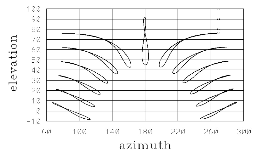
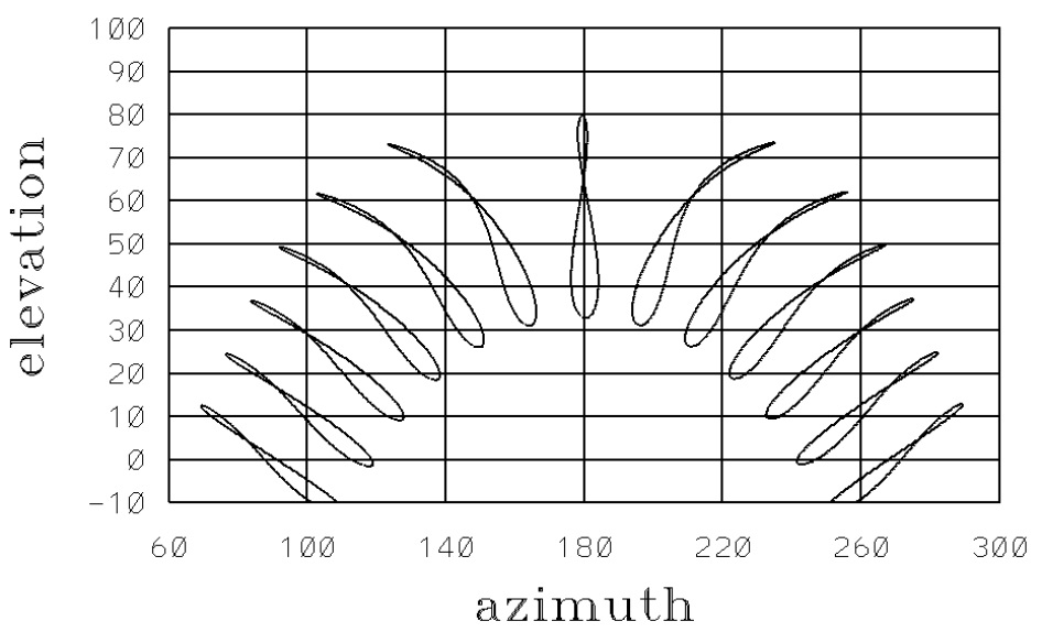
Figure 6 shows the analemma calculated for an observer located in the Holy city of Mecca, at latitude $\delta ={21.42}^{\circ }$ for the year 2025. Here, the left panel shows the analemma at 10:00 A.M., the middle panel shows the analemma at noon, and the right panel shows the analemma at 4:00 P.M., local time at the location. Whereas, Figure 7 shows several analemmas for the Holy city of Mecca with a time difference of one hour from 6 A.M. to 11 A.M. (towards the left of Figure 7) and from 1 P.M. to 6 P.M. The central analemma is for local noon. It is observable that the analemmas before local noon are tilted towards the left, and those after local noon are tilted towards the right. The size of the analemma increases with the increasing angle of elevation, i.e., towards local noon. Figure 8 presents the analemmas for Islamabad. For the reason of similarity with Figure 7, the hourly analemmas for Mexico City are not presented. It may be recalled that the latitudes of Mexico and Mecca are 19.4 and 21.42 degrees, respectively.

4. Results and Discussion

In our earlier companion papers [5, 6], diverse computational methodologies were presented to calculate the position of the Sun in the sky of an observer located on Earth that is revolving around the Sun in an elliptic orbit, as well as rotating around its axis. After precisely locating the North Star, the azimuthal angle, the position vector from the Earth to the Sun, $\gamma \left(t\right)$, the elevation angle, $\alpha \left(t\right)$, and the declination angle, $\beta \left(t\right)$, as a function of time, were obtained by using a numerical approach and the PSA algorithm [8, 9, 10, 11, 12].

In this paper, we have calculated the solar position for all days of the year 2025. It may be mentioned here that the analemmas for all the years having 365 days are the same; hence, the analemmas for leap years having 366 days would be different (not presented here). The calculations were done for an observer located at three distinct locations in the northern hemisphere, viz. Mexico City, Islamabad, and the holy city of Mecca (corresponding to the latitudes $\delta ={19.4}^{\circ }$, ${33.74}^{\circ }$, and ${21.42}^{\circ }$, respectively).

Our study examines solar analemma patterns across three representative cities spanning different latitudes: Mexico City (19.4^∘N), Islamabad (33.7^∘N), and Mecca (21.4^∘N). Initial analysis focuses on three key observation times—morning (10:00 A.M. local time), local noon, and afternoon (4:00 P.M. local time)—revealing characteristic number-eight trajectories for each location. For enhanced temporal resolution, Figures 6 and 7 present comprehensive hourly analemma progressions from 6:00 A.M. to 6:00 P.M. specifically for Mecca and Islamabad, illustrating the continuous evolution of solar azimuth and elevation angles throughout the day. Although Mexico City exhibits analogous diurnal patterns (demonstrated in Figure 4), we deliberately exclude its hourly plots to prevent redundancy, given their close similarity to Mecca's profiles in Figure 6. Of particular astronomical significance is the Islamabad dataset (Figure 7), where the Sun's maximum elevation always remains below the zenith (), a direct consequence of the city's position north of the Tropic of Cancer (23.5^∘N) where the solar declination never equals the local latitude. This latitudinal effect creates unique observational constraints compared to lower-latitude locations.

5. Conclusions

From the results presented in this work, it could be concluded that the shapes of the analemmas are quite similar at all the locations in the northern hemisphere. The shape at local noon resembles like the symbol "8" with upper part much smaller than the lower one [2, 8]. The analemmas before noon are tilted towards left and those for the afternoon are tilted towards right. Our results also confirm the fact that when the sun reaches the zenith position (directly overhead) for an observer located at a latitude lower than the Tropic of Cancer (23.5°N), at local noon on the solstice day i.e. June 21, for the northern hemisphere.

The information included in this paper should be considered as an important source of reference for the solar energy engineers, who need to accurately know the position of sun throughout the year, for calculating the incoming solar irradiance, shadows and the atmospheric temperature for green energy applications.