Soret and Dufour Effects in Computational Analysis of Assisting and Opposing Stagnation Point Flow of Viscoelastic Fluid

Amir Abbas; Qurat ul Ain; Asifa Ilyas; Laraib Kiran; Mdi Begum Jeelani

doi:10.62762/CEHT.2025.786259

1. Introduction

In recent years, the concept of non-Newtonian fluids has sparked a flurry of active research, as the fluids course represents, methodically, many modern significant fluids such as artificial fibres and microfilm in production. Due to their many applications in industries and engineering, the research community has focused extensively on such fluids. The diffusion-thermo effect, also known as the Dufour composition, is the driving mass flux that causes the temperature flow. The thermal-diffusion or Soret configuration involves temperature slopes that cause mass flows. The Soret and Dufour effects have been applied in a variety of practical applications, including chemical engineering and geology. Stagnation point is a term used in hydrodynamics to describe a place within a fluid region when the fluid regional velocity is zero. Cooling of the atomic pile, supercooling of the thermionic tube, polymer ejection, drawing of plastic sheets, wire drawing, and many more hydrodynamic processes in engineering applications are all examples of stagnation point flow uses.

Abbasi et al. [1] investigated a nanofluid's magnetohydrodynamic (MHD) doubly laminated mixed convection Maxwell flow. The structure of coupled convection flow with nanofluid inclusion filled through a lid driven liable form was presented by Abu-Nada et al. [2]. Ahmad and Ioan Pop [3] investigated nanofluid mixed convection flow across an upright uniform surface immersed inside an absorbent tube. Ahmed et al. [4] investigated the rotational stagnation-point flow caused by a Maxwell microfluid passing over a porous disc that was shrinking and extending. As a result of this, Arafa et al. [5] used the homotopy analysis technique to develop a biological population model. Bachok et al. [6] examined stagnation point flow with reference to stretching/contracting surface. Balci et al. [7] proposed a rectification tensor to viscoelastic fluid template of uniform factorization. Using a rigorous numerical approach, Bhatti et al. [8] presented a stagnation point flow above this porous contracting sheet undergoing superemacy on MHD. Using the homotopy analysis mechanism on MHD flow above a stretching absorptive sheet, Daniel et al. [9] investigated the heat radiation and buoyancy effects. The homotopy analysis method was suggested by Dehghan et al. [10] for resolving nonlinear fractional partial equations. Hayat et al. [11] presented a viscoelastic fluid flow in a stagnation point with mixed convection on a vertical surface in a viscoelastic fluid flow. Hayat et al. [12] used thermophoresis to explore the radiant and joule heating reactions of mass and heat conduct inside the MHD region using an Oldroyd-B fluid. The thermal radiation impact of marangoni convection along a water carbon nanofluid was proposed by Hayat et al. [13]. He et al. [14] presented a fractional-order hyperchaotic technique that might be used in a similar Homotopy analysis procedure. In the stagnation point, Ishak et al. [15] presented a compressing sheet in a micropolar zone.

Mixed convection in various forms of nanofluid enclosures was discussed by Izadi et al. [16]. The magneto walter-B nano liquid with mixed convection flow of nonlinear radiation was predicted by Khan et al. [17]. Khan [18] looked at the unsteady MHD flow of an expanding surface and also talked about the free convection boundary-layer flow of nanofluid with radiant thermals and viscid dissipation effects. Khan et al. [19] examined a self-contained MHD flow with a stagnation point referring to a nanofluid with varying viscidity applied on an outstretched sheet with radiation effects. By the occurrence of transpiration as well as chemical reaction, Mabood et al. [20] concentrated the mix mass and heat transfer by stagnation point flow of MHD above the porous elongating plate. Majeed et al. [21] studied a boundary layer heat transfer flow employing the features of ferromagnetic viscoelastic fluid flow in two dimensions past a stretched sheet. The simulation approach of viscoelastic fluid flows of lattice Boltzmann was anticipated by Malaspinas et al. [22]. The approach for addressing a nonlinear second-order boundary value problem with a new spectral-homotopy was discovered by Motsa et al. [23]. In MHD viscoelastic flow, Prasad et al. [24] looked at heat transmission in the presence of variable viscosity above an elongated sheet. Prasad et al. [25] investigated free convection mass and heat transfer in MHD flow with thermal radiation effects from a sphere and a changeable porosity structure.

The study focusing on the numerical evaluation of viscoelstic fluid flow over a vertical surface for the aiding and opposing situations in the presence of Soret and Dufour effects is obvious from the preceding literature survey. The study utilizes stream functions and similarity variables to transform the governing partial differential equations into ordinary differential equations. MATLAB software built-in solver bvp4c is employed to obtain numerical and graphical profiles for mass transport, temperature, and velocity. Additionally, the software is used to compute the mass transfer rate, and skin friction coefficient under various physical conditions, providing a comprehensive analysis of the system's behavior. The mathematical modelling, as well as numerical solutions in the form of the above mentioned, will be provided in depth in the fourth section.

2. Flow Analysis

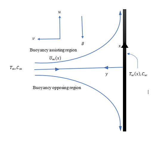
Consider a viscous, two-dimensional, incompressible boundary layer stagnation point flow in a viscoelastic fluid over a vertical surface with Soret and Dufour effects. The temperature of the surface is $T_{w}(x)$ with $T_{w}(x)>T_{\infty}(x)$ being the condition. Here free stream temperature is given by $T_{\infty}(x)$ . The flow configuration is shown in Figure 1. The mass concentration at surface is $C_{w}(x)$ with condition $C_{w}(x)>C_{\infty}(x)$ , where $C_{\infty}(x)$ is free stream mass concentration. By following [11] the flow equations equation:

Figure 1 Flow Configuration.

\frac{\partial u}{\partial x}+\frac{\partial v}{\partial y}=0

\begin{split}u\frac{\partial u}{\partial x}+v\frac{\partial u}{\partial y}&=U% \frac{dU}{dx}+\nu\frac{\partial^{2}u}{\partial y^{2}}\\ &+k_{0}\left(u\frac{\partial^{3}u}{\partial x\partial y^{2}}+\frac{\partial u}% {\partial x}\frac{\partial^{2}u}{\partial y^{2}}\right.\\ &\left.+\frac{\partial u}{\partial y}\frac{\partial^{2}v}{\partial y^{2}}+\nu% \frac{\partial^{3}u}{\partial y^{3}}\right)\\ &\pm g\beta_{T}\left(T-T_{\infty}\right)\\ &\pm g\beta_{C}\left(C-C_{\infty}\right)\end{split}

u\frac{\partial T}{\partial x}+v\frac{\partial T}{\partial y}=\alpha\frac{% \partial^{2}T}{\partial y^{2}}+\frac{D_{m}k_{T}}{C_{s}C_{p}}\frac{\partial^{2}% C}{\partial y^{2}}

u\frac{\partial C}{\partial x}+v\frac{\partial C}{\partial y}=D_{m}\frac{% \partial^{2}C}{\partial y^{2}}+\frac{D_{m}k_{T}}{T_{m}}\frac{\partial^{2}T}{% \partial y^{2}}

Subject to the boundary conditions

\begin{split}u&=0,\quad v=0,\quad T=T_{w},\quad C=C_{w}\quad\text{at}\quad y=0% ,\\ u&\rightarrow U_{\infty},\quad\frac{\partial u}{\partial y}\rightarrow 0,\quad T% \rightarrow T_{\infty},\quad C\rightarrow C_{\infty}\quad\\ &\text{as}\quad y\rightarrow\infty\end{split}

where $x$ and $y$ horizontal and normal coordinates respectively. Here, along $x$ and $y$ axis, the velocity components are taken as $u$ and $v$ respectively. The notations $g$ , $\nu$ , $k_{0}$ and $\alpha$ gives the gravitational acceleration, kinematic viscosity, viscoelastic parameter and thermal diffusivity respectively. Where $T$ and $C$ is the temperature of the fluid and concentration at any point in the flow field respectively. The symbols $T_{\infty}$ and $C_{\infty}$ is the temperature at the free stream and concentration at the free stream respectively. The representations $D_{m}$ , $\beta_{C}$ , $k_{T}$ , $T_{m}$ is the mass diffusivity, concentration expansion coefficient, thermal diffusion ratio, and mean fluid temperature respectively. The physical parameters $\beta_{T}$ , $C_{s}$ and $C_{p}$ and is the thermal expansion coefficient, concentration susceptibility and specific heat at constant pressure respectively.

3. Solution Methodology

This section is confined to the method of solution adopted to find out the numerical solution of the flow model. The partial differential equations (1-4), subject to the boundary conditions (5), are transformed into ordinary differential equations and then solved using bvp4c, a built-in numerical solver. The whole solution methodology is elaborated in the following subsection.

3.1 Stream Function Formulation

The solution of the partial differential equations using the method directly on them is difficult; therefore, if we convert them into ordinary differential equations, then the numerical technique will be used. For the conversion from PDEs to ODEs, the stream function formulation given in Eq. (1) is utilized.

\begin{split}\eta&=\sqrt{\frac{a}{\nu}}y,\\ u&=axf^{\prime}(\eta),\\ v&=-\sqrt{a\nu}f(\eta),\\ \theta(\eta)&=\frac{T-T_{w}}{T_{w}-T_{\infty}},\\ \phi(\eta)&=\frac{C-C_{\infty}}{C_{w}-C_{\infty}}\end{split}

Now by using the stream function formulation, we have the following transformed boundary layer equations.

\begin{split}f^{\prime\prime\prime}+ff^{\prime\prime}-f^{\prime 2}+1&=K\left(f% ^{\prime\prime 2}-2f^{\prime}f^{\prime\prime\prime}+ff^{\prime\prime\prime% \prime}\right)\\ &\pm\lambda_{T}\theta(\eta)\\ &\pm\lambda_{c}\phi(\eta)=0\end{split}

\begin{split}f^{\prime}\theta-f\theta^{\prime}&=\frac{1}{\Pr}\theta^{\prime% \prime}\\ &=Du\phi^{\prime\prime}(\eta)\end{split}

f^{\prime}\phi-f\phi^{\prime}-\frac{1}{Sc}\phi^{\prime\prime}=Sr\theta^{\prime% \prime}(\eta)

Flow conditions

\begin{split}f(0)&=f^{\prime}(0)=0,\ \theta(0)=1,\ \phi(0)=1\ \text{as}\ y% \rightarrow 0\\ f^{\prime}(\infty)&=1,f^{\prime\prime}(\infty)=0,\ \theta(\infty)=0,\ \phi(% \infty)=0\ \text{as}\ y\rightarrow\infty\end{split}

where

\displaystyle K=\frac{k_{0}a}{\rho},\Pr=\frac{\upsilon}{\alpha},Sc=\frac{% \upsilon}{D_{m}},

\displaystyle Sr=\frac{D_{m}k_{T}(T_{w}-T_{\infty})}{T_{m}\nu(C_{w}-C_{\infty}% )},

\displaystyle Du=\frac{D_{m}k_{T}(C_{w}-C_{\infty})}{C_{s}C_{p}\nu(T_{w}-T_{% \infty})},

\displaystyle\lambda_{T}=\frac{Gr_{T}}{Re_{x}^{2}},\lambda_{C}=\frac{Gr_{C}}{% Re_{x}^{2}},

are viscoelastic parameter, Prandtl number, Schmidt number, Soret number, Dufour number, mixed convection parameter and the modified mixed convection parameter respectively.

3.2 Solution Technique

The numerical outcomes are obtained by solving the Eqs. (2-4) with boundary conditions given in (5). Numerical solutions Eqs. (2-4) are also given in tabular forms. A numerical simulation is performed by means of solver bvp4c. In simulation of numerical solutions $\eta_{\infty}=8$ and bvp4c is based on finite difference method that uses three-stage Lobatoo formula. The continuous solutions decided the mesh selection and error control. In this technique of collocation mesh interval is divide the interval into subintervals. The initial mesh and initial approximation are provided to the mesh points for final solution of the equations. Eqs. (2-4) subject to the boundary conditions (5) are in higher order, so firstly they are converted to set of first order differential equations. Equations are as follow:

\begin{split}f&=\Gamma(1),\quad f^{\prime}=\Gamma(2),\quad f^{\prime\prime}=% \Gamma(3),\\ f^{\prime\prime\prime}&=\Gamma(4),\quad\theta=\Gamma(5),\quad\theta^{\prime}=% \Gamma(6),\\ \phi&=\Gamma(7),\quad\phi^{\prime}=\Gamma(8)\end{split}

\begin{split}f^{(iv)}&=\Gamma\Gamma 1=\frac{1}{K*\Gamma(1)}\left(\Gamma(4)+% \Gamma(1)*\Gamma(3)-\Gamma(2)^{2}+1\right)\\ &\quad-K\left(\Gamma(3)^{2}-2*\Gamma(2)*\Gamma(4)\right)\pm\lambda_{T}\Gamma(5% ),\\ &\quad\pm\lambda_{C}\Gamma(7)-M*(\Gamma(2)-1)-K_{1}*\Gamma(2)\\ &\quad-F*(\Gamma{(2)-1)}^{2}\end{split}

\begin{split}\theta^{\prime\prime}&=\Gamma\Gamma 2=-Pr*\left(\Gamma(2)*\Gamma(% 5)-\Gamma(1)*\Gamma(6)\right)\\ &\quad+Du*\Gamma\Gamma 3\end{split}

\begin{split}\phi^{\prime\prime}&=\Gamma\Gamma 2=-Sc*\left(\Gamma(2)*\Gamma(7)% -\Gamma(1)*\Gamma(8)\right)\\ &\quad+Sr*\Gamma\Gamma 2\end{split}

Subject to the boundary conditions

\begin{split}\Gamma(1)&=\Gamma(2)=0,\ \Gamma(5)=1,\ \Gamma(7)=1\ \text{at}\ % \eta=0\\ \Gamma(2)&\rightarrow 1,\ \Gamma(3)\rightarrow 0,\ \Gamma(5)\rightarrow 0,\ % \Gamma(7)\rightarrow 0\ \text{as}\ \eta\rightarrow\infty\end{split}

The equations (6-10) are put into the algorithm of bvp4c solver and then required solutions for an appropriate choice parameter involved in the problem are obtained. These solutions in graphical and tabular form are presented in the next sections.

Figure 2 Consequences of

\lambda_{T}

on

f^{\prime}(\eta)

\theta(\eta)

\phi(\eta)

.

Figure 3 Consequences of

\lambda_{C}

on

f^{\prime}(\eta)

\theta(\eta)

\phi(\eta)

.

4. Results and Discussion

The current discussion is focused on the behavior of unknown physical variables such as velocity profile $f^{\prime}$ , temperature profile $\theta$ , and mass concentration $\phi$ , as well as their derivatives, such as skin friction $f^{\prime\prime}(0)$ , rate of heat transfer $\theta^{\prime}(0)$ and rate of mass transfer $\phi^{\prime}(0)$ for various values of involved parameters. To investigate the impact of several physical factors on velocity, temperature, and concentration profiles, such as mixed convection parameters $\lambda_{T}$ , modified mixed convection parameter $\lambda_{T}$ , viscoelastic parameter $K$ , Prandtl number $P r$ , Soret number $S r$ , and Schmidt number $S c$ , Dufour number $D u$ . Figures 2, 3, 4, 5, 6, 7 and 8 show the plots for various parametric settings. For your convenience, the variation of all physical parameters on the velocity function, temperature, and concentration profile against $\eta$ are shown for assisting and opposing flows respectively.

Figure 4 Consequences of

K

on

f^{\prime}(\eta)

\theta(\eta)

\phi(\eta)

.

Figure 5 Consequences of

D u

on

f^{\prime}(\eta)

\theta(\eta)

\phi(\eta)

.

Figure 6 Consequences of

S r

on

f^{\prime}(\eta)

\theta(\eta)

\phi(\eta)

.

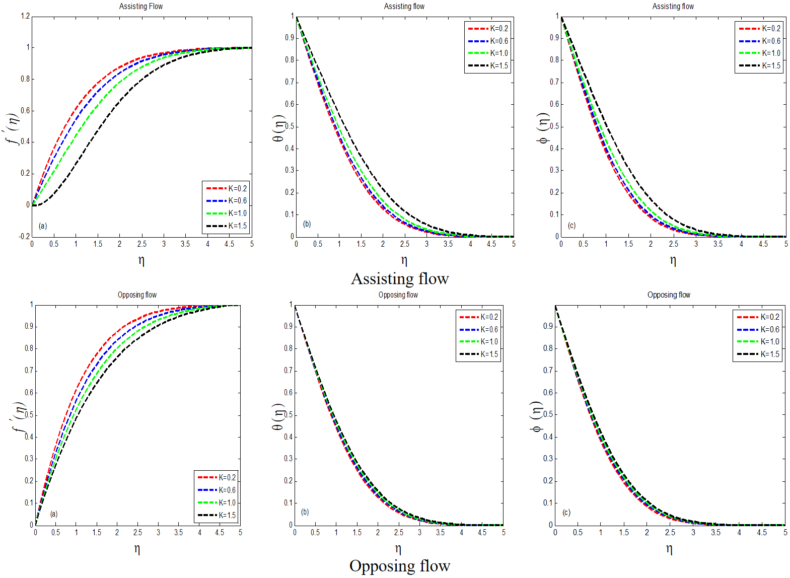
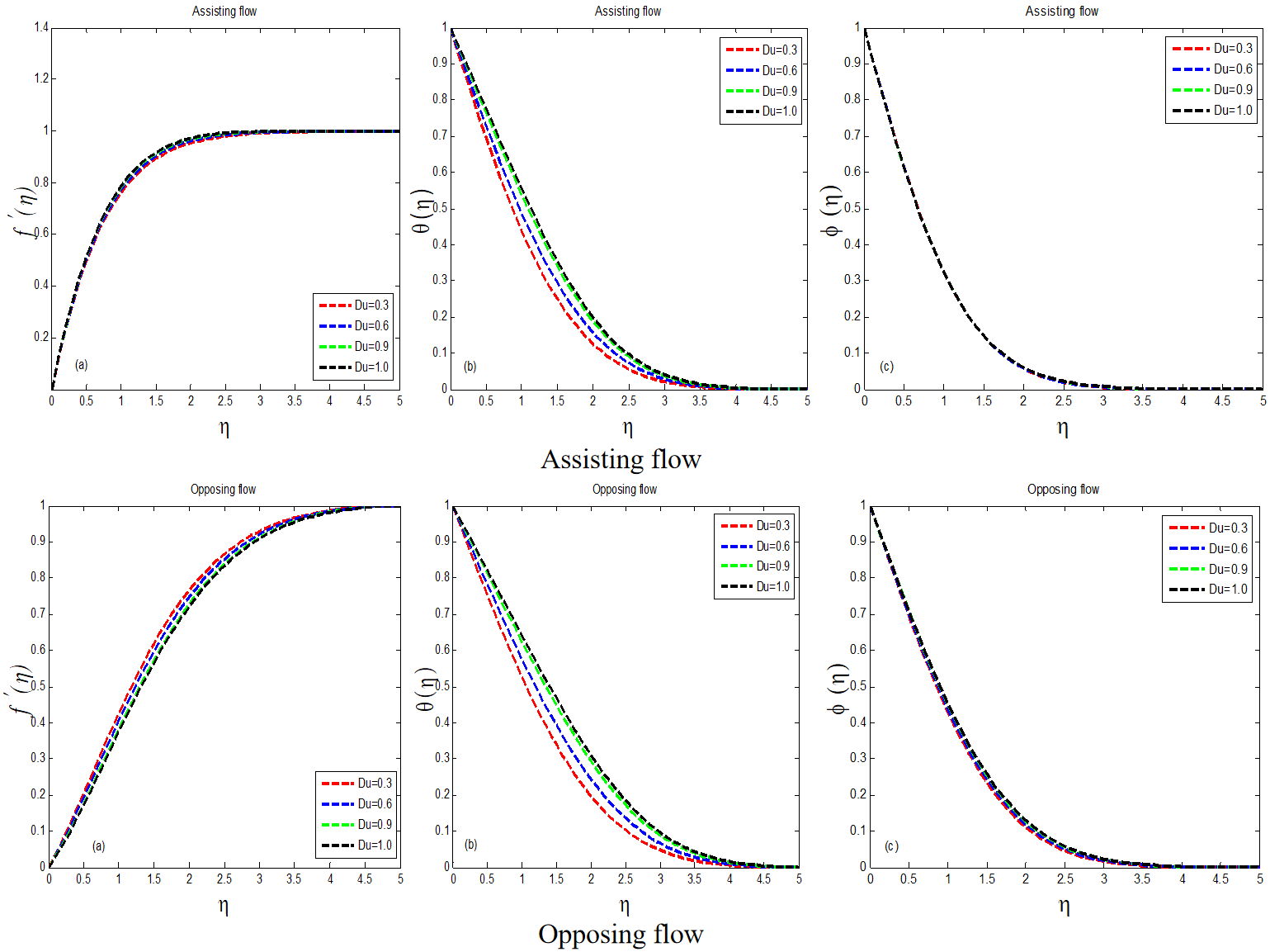
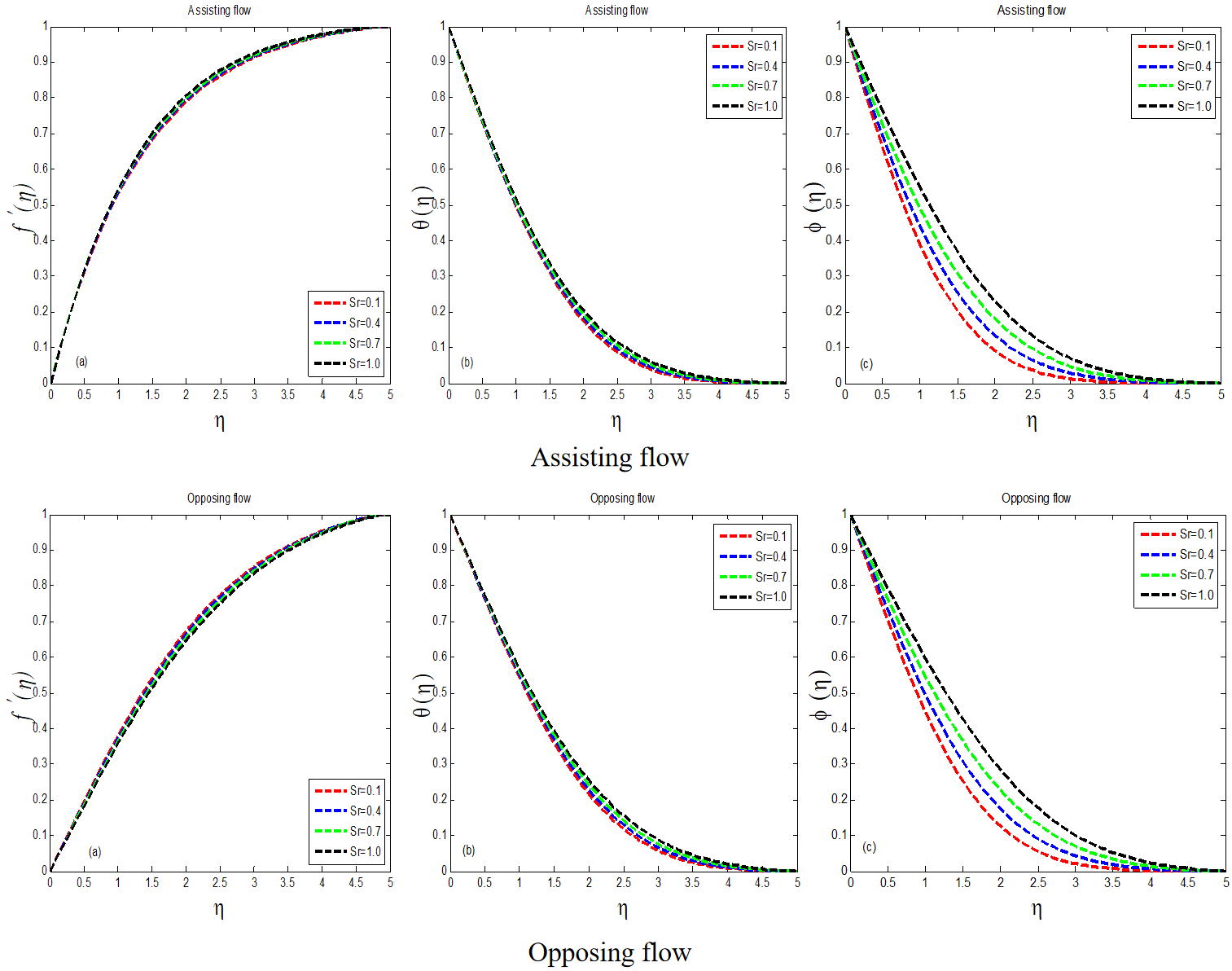
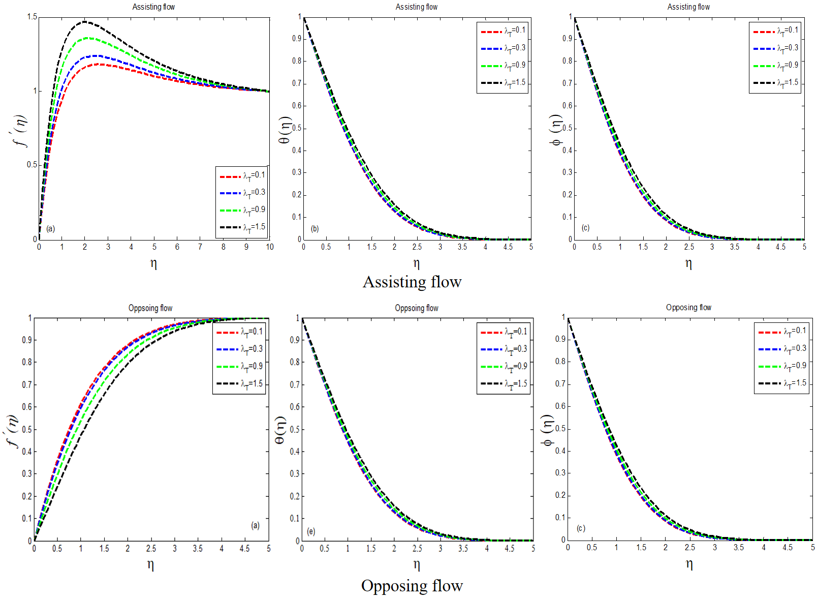
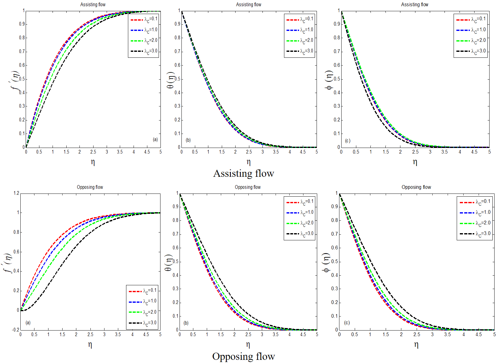
Figure 2 depicts the results of $f^{\prime}(\eta)$ against $\lambda_{T}$ for aiding and opposing flows, showing that $f^{\prime}(\eta)$ rises for assisting flow and falls for opposing flow. The behavior of the temperature and concentration profile with the impact of $\lambda_{T}$ is shown in Figure 2. Temperature and concentration profiles grow as the value of $\lambda_{T}$ increases, as shown in the graph. Both helpful and opposing flows have a very modest difference in and. Figure 2 show the behaviour of the fluid velocity temperature and concentration field as the parameter $\lambda_{T}$ is increased. As a result, we can observe that the impact of $\lambda_{T}$ on $f^{\prime}(\eta)$ and the impact of $\lambda_{T}$ on and are inverted. The graph clearly shows a decrease in velocity field and an increase in temperature and mass concentration. Figure 3 show the results for velocity distribution, fluid temperature, and concentration field for various values of $\lambda_{C}$ , and the peculiarities of the velocity profile under the action of $\lambda_{C}$ are highlighted. In the flow field, the $\lambda_{C}=0.1$ velocity profile offers a high value, while the $\lambda_{C}=3.0$ velocity profile gives a short value. The graph shows that when the value of $\lambda_{C}$ increases, the projected quantity decreases, and the flashout effect of various increasing values of $\lambda_{C}$ on the temperature profile. The temperature field is reduced at the minimum value of $\lambda_{C}$ , and the temperature field is increased at the maximum value of $\lambda_{C}=3.0$ . Because the temperature profile and $\lambda_{C}$ have a direct relationship in this scenario, the thermal boundary layer is increased. While the phenomena are the same, there are some differences in assisting and opposing flow. The mass concentration for various values of $\lambda_{C}$ is shown in Figure 3.

Figure 7 Consequences of

\Pr

on

f^{\prime}(\eta)

\theta(\eta)

\phi(\eta)

.

Figure 8 Consequences of

S c

on

f^{\prime}(\eta)

\theta(\eta)

\phi(\eta)

.

For rising values of the physical viscoelastic parameter, the velocity field is seen in Figure 4 . This graph indicates that when $f^{\prime}$ decreases in assisting flow, the value of $K$ increases. Both $f^{\prime}(\eta)$ and $K$ have an inverse relationship. In both aiding and opposing flows, greater values of $K$ in the velocity profile show some difference. Figure 4 show the effect of temperature and mass concentration on $K$ . For both scenarios of flow, augmenting $K$ results in $\theta(\eta)$ and $\phi(\eta)$ , although the opposite is true for $f^{\prime}(\eta)$ . Figure 5 depicts the velocity distribution as a function of the Dufour number. Other unquantifiable factors, on the other hand, remain constant. According to the graph, the recommended variable Dufour number $D u$ increases at $D u$ =1.0 and decreases at $D u$ =0.3. There is a distinction in velocity for both values of the dufour number. For varying values of the dufour number, all curves in the assisting flow display nearly identical behavior with minor differences. When compared to assisting flow, the behavior of velocity for growing $D u$ values differs in opposing flow. When we consider many values of the Dufour number, Figure 5 shows the temperature in detail. The results indicate that reducing the value of $D u$ leads to an increase in $\theta(\eta)$ . It is maximum at $D u$ =1.0 and minimised at $D u$ =0.3. When we compare the activities of $\theta(\eta)$ for both sorts of flows, we can see that they act in the same way. When we improve the Dufour number, the manner of mass concentration $\phi(\eta)$ is depicted in Figure 5. In the assisting flow, just a single curve is obtained for the number of values of the Dufour parameter. When variation is offered to the Dufour number in opposing flow, a slight gap is perceived.

Table 1 Consequences of

\lambda_{T}

on

f^{\prime\prime}(0)

\theta^{\prime}(0)

\phi^{\prime}(0)

.

\lambda_{T}

f^{\prime\prime}(0)

-\theta^{\prime}(0)

-\phi^{\prime}(0)

Assistant

flow

0.1

0.94579

0.64135

0.7275

0.3

0.9915

0.64799

0.73543

0.9

1.12266

0.66639

0.75735

1.5

1.24628

0.68291

0.77701

Opposing

flow

0.1

0.85614

0.6283

0.71187

0.3

0.80681

0.62071

0.70279

0.9

0.64892

0.59522

0.67223

1.5

0.47076

0.56386

0.63449

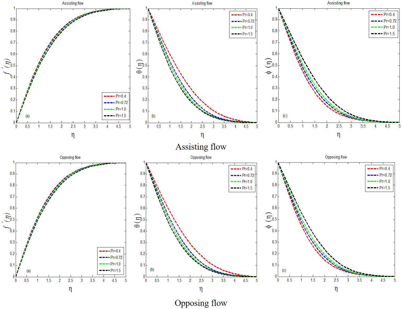
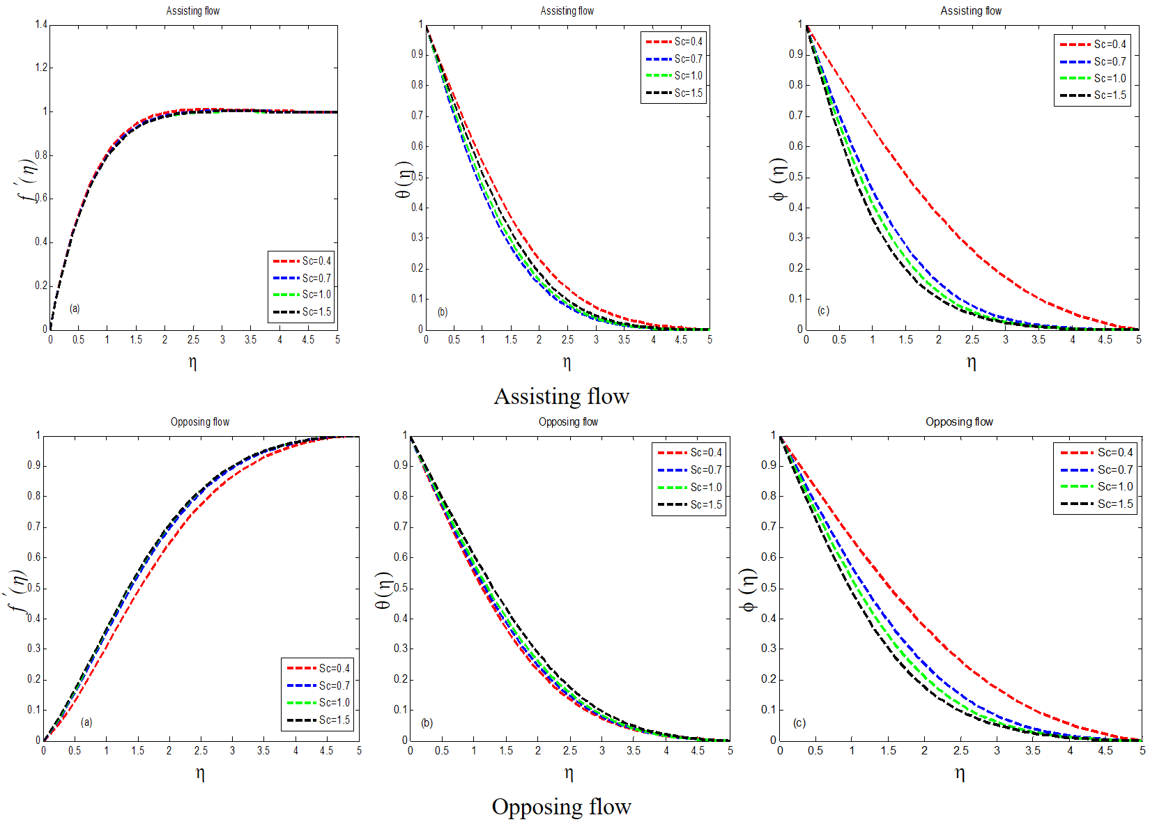
The influence of soret number $S r$ on velocity profile is shown in Figure 6. In helping flow, the curve of $f^{\prime}$ shortens at $S r$ =0.1 and the velocity field increases at $S r$ =1.0, whereas in opposing flow, the situation is reversed. Figure 6 show how temperature $\theta(\eta)$ and mass concentration $\phi(\eta)$ behave under the impact of soret number. Temperature and mass concentration play a role in expanding $S r$ . As a result, the thickness of the thermal boundary layer raised. The same thing happens in both aiding and opposing flows. With the execution of the prandtl number, Figure 7 focuses the physical velocity field. In the flow domain, the graph illustrates many values of proposed quantity rise at $P r$ =0.4 and decrease at $P r$ =1.5. Figure 7 show the temperature $\theta(\eta)$ and mass concentration $\phi(\eta)$ with Prandtl number dominance. It is worth noting that as Prandtl number increases in both opposing and assisting flows, $\theta(\eta)$ and $\phi(\eta)$ decrease. The thickness of the thermal boundary layer decreases as $P r$ increases. The velocity and temperature profiles for a variety of Schmidt numbers are depicted in Figure 8.

These graphs show that the velocity and temperature fields decrease as $S c$ increases. In helping flow, the value of $S c$ =0.4 velocity $f^{\prime}(\eta)$ and temperature continues to rise, whereas the value of $S c$ =1.5 velocity $f^{\prime}(\eta)$ and temperature continues to fall with a minor difference. In the opposing flow, however, the value of $S c$ =0.4 indicates a lesser value of $f^{\prime}(\eta)$ and $\theta(\eta)$ , whereas $S c$ =1.5 indicates a high value of $f^{\prime}(\eta)$ and $\theta(\eta)$ . In aiding and opposing flows, the behaviour of $f^{\prime}(\eta)$ and $\theta(\eta)$ with the impression of Schmidt number is obverse to each other. The various outcomes of Schmidt number on mass concentration $\phi(\eta)$ are shown in Figure 8. Innumerable values of Schmidt number show the two of them supporting and opposing flow in the same way. The concentration field produces an inflated curve when $S c$ =0.4, but a deflated curve when $S c$ =1.5.

Table 2 Consequences of

\lambda_{C}

on

f^{\prime\prime}(0)

\theta^{\prime}(0)

\phi^{\prime}(0)

.

\lambda_{C}

f^{\prime\prime}(0)

-\theta^{\prime}(0)

-\phi^{\prime}(0)

Assistant

flow

0.1

0.94579

0.64135

0.7275

1

1.1229

0.6651

0.75596

2

1.30383

0.68784

0.78314

3

1.47212

0.7078

0.80694

Opposing

flow

0.1

0.85614

0.6283

0.71181

1

0.64824

0.59688

0.67405

2

0.3715

0.54961

0.61686

3

-0.04342

0.46033

0.50765

The behaviour of the derivatives of mass concentration, velocity profile, and temperature profile, which are the rate of mass transfer $\phi^{\prime}(0)$ , skin friction $f^{\prime\prime}(0)$ , and heat transfer rate $\theta^{\prime}(0)$ for various parameters, is shown in Tables 1, 2, 3, 4, 5, 6 and 7. Tables 1 and 2 show the obtained results for $f^{\prime\prime}(0)$ , $\theta^{\prime}(0)$ $\phi^{\prime}(0)$ upsurges whenever the modified mixed convection parameter $\lambda_{C}$ and mixed convection parameter $\lambda_{T}$ develop well in helping flow but opposite relation occurs in opposing flow, for budding values of the above-mentioned material attributes. The physical parameters $\lambda_{T}$ and $\lambda_{C}$ behave in the same way. Significant features like $f^{\prime\prime}(0)$ , $\theta^{\prime}(0)$ , and $\phi^{\prime}(0)$ compressed in aiding and opposing flows for advanced values of viscoelastic parameter $K$ , as shown in Table 3.

Table 3 Consequences of

K

on

f^{\prime\prime}(0)

\theta^{\prime}(0)

\phi^{\prime}(0)

.

K

f^{\prime\prime}(0)

-\theta^{\prime}(0)

-\phi^{\prime}(0)

Assistant

flow

0.2

0.94579

0.64135

0.7275

0.6

0.8336

0.62093

0.70351

1

0.75137

0.60414

0.68387

1.5

0.67513

0.58695

0.66386

Opposing

flow

0.2

0.85614

0.6283

0.71187

0.6

0.75061

0.60772

0.68772

1

0.6736

0.59086

0.66801

1.5

0.60254

0.57365

0.64797

Table 4 Consequences of

D u

on

f^{\prime\prime}(0)

\theta^{\prime}(0)

\phi^{\prime}(0)

.

D u

f^{\prime\prime}(0)

-\theta^{\prime}(0)

-\phi^{\prime}(0)

Assistant

flow

0.3

1.31385

0.63204

0.81372

0.6

1.33316

0.5537

0.81595

0.9

1.35271

0.47367

0.81812

1

1.35929

0.44662

0.81884

Opposing

flow

0.3

0.35472

0.50207

0.62756

0.6

0.31965

0.43901

0.61431

0.9

0.28273

0.37799

0.60006

1

0.26998

0.35817

0.59505

Under the influence of $K$ , the numerical findings of $f^{\prime\prime}(0)$ , $\theta^{\prime}(0)$ , and $\phi^{\prime}(0)$ reveal identical actions for both types of flows. The derivatives of mass concentration, velocity profile, and temperature profile for Dufour number $D u$ are shown in Table 4. When the Dufour number increases, the skin friction and mass transfer rate increase, while the heat transfer rate decreases. We get to the conclusion that they have the inverse relationship. When we look at the second type of flow, opposing flow, under the stimulation of the Dufour number $D u$ , we see that the measurable properties $f^{\prime\prime}(0)$ , $\theta^{\prime}(0)$ , and $\phi^{\prime}(0)$ are lowered when the Dufour number is increased.

Table 5 Consequences of

S r

on

f^{\prime\prime}(0)

\theta^{\prime}(0)

\phi^{\prime}(0)

.

S r

f^{\prime\prime}(0)

-\theta^{\prime}(0)

-\phi^{\prime}(0)

Assistant

flow

0.1

0.74342

0.54756

0.6976

0.4

0.74914

0.54182

0.62892

0.7

0.7551

0.53567

0.55772

1

0.76132

0.52905

0.48371

Opposing

flow

0.1

0.38926

0.48549

0.60964

0.4

0.38019

0.47633

0.54759

0.7

0.37054

0.46668

0.4845

1

0.36022

0.4565

0.42033

Table 6 Consequences of

P r

on

f^{\prime\prime}(0)

\theta^{\prime}(0)

\phi^{\prime}(0)

.

P r

f^{\prime\prime}(0)

-\theta^{\prime}(0)

-\phi^{\prime}(0)

Assistant

flow

0.4

1.14857

0.46591

0.70168

0.72

1.15876

0.55524

0.65037

1

1.16804

0.60791

1.5

1.18617

0.67304

0.53268

Opposing

flow

0.4

0.61448

0.41822

0.61366

0.72

0.60077

0.48891

0.56674

1

0.58818

0.52816

1.5

0.56321

0.57164

0.46053

Table 7 Consequences of

S c

on

f^{\prime\prime}(0)

\theta^{\prime}(0)

\phi^{\prime}(0)

.

S c

f^{\prime\prime}(0)

-\theta^{\prime}(0)

-\phi^{\prime}(0)

Assistant

flow

0.4

1.3961

0.66021

0.50838

0.7

1.37618

0.61582

0.60778

1

1.3674

0.57763

0.67817

1.5

1.36377

0.5196

0.76489

Opposing

flow

0.4

0.196

0.46725

0.37703

0.7

0.23647

0.4543

0.44933

1

0.25403

0.43575

0.4988

1.5

0.2613

0.40068

0.55478

Table 5 shows how the behaviour of helping flow changes when the Soret number $S r$ increases, while the heat transfer rate and mass transfer rate decrease. When we compare the numerical phenomena of assisting flow with opposing flow, we find that with bigger values of Soret number $S r$ in opposing flow, $f^{\prime\prime}(0)$ , $\theta^{\prime}(0)$ and $\phi^{\prime}(0)$ decrease. Table 6 shows the numerical results of $f^{\prime\prime}(0)$ , $\theta^{\prime}(0)$ and $\phi^{\prime}(0)$ when Prandtl number $P r$ is used. In assisting flow, the values of Prandtl number $P r$ , skin friction and the rate of heat transfer increased, while the rate of mass transfer decreased, and in opposing flow, the values of Prandtl number $P r$ skin friction $f^{\prime\prime}(0)$ , and rate of mass transfer $\phi^{\prime}(0)$ decreased, while the rate of heat transfer increased. In assisting flow, the material properties $f^{\prime\prime}$ , $\theta^{\prime}(0)$ lowered and $\phi^{\prime}(0)$ abated as the Schmidt number $S c$ increased, but in opposing flow, the material properties $f^{\prime\prime}(0)$ expanded and the rate of heat transfer decreased as the Schmidt number $S c$ increased.

5. Conclusion

In this study, we study the mixed convection stagnation point flow in viscoelastic fluid in the presence of Soret and Dufour effects over a vertical surface was numerically derived for different dimensionless factors. The Numerical results for the physical parameters seemed in a main flow domain, such as the physical dimensionless parameters performing in the main equations are Schdmit Number $S c$ , Prandtl number $P r$ , Soret number $S r$ and Dufour number $D u$ were painted. The experimental results demonstrated the performance of the baseline model and its effectiveness in flow control. The main verdicts about this theoretical study are:

From results for $f^{\prime}(\eta)$ , it was examined that the $f^{\prime}(\eta)$ bloated for rising values of $S r$ but condensed when $\lambda_{T}$ , $\lambda_{C}$ , $K$ , $S c$ , $D u$ and $P r$ were augmented.
This was an experiential effect which shows that the answers about the temperature field that this physical thing was improved when $\lambda_{T}$ , $\lambda_{C}$ , $K$ and $S r$ was amplified and reduced when $P r$ , $D u$ , $S c$ were increased.
The conclusions made for the mass concentration design for emerging values of $\lambda_{T}$ , $K$ , $S r$ and $S c$ abortive as $\lambda_{C}$ , $D u$ and $P r$ were enhanced.
It was observed from the graphical study that velocity profile increases for growing values of $S c$ yet concentrates for the amplification in values of $\lambda_{T}$ , $\lambda_{C}$ , $K$ , $D u$ , $P r$ and $S r$ .
The judgment about temperature profile gave the experiential results that such physical material was upgraded by the amplification in $\lambda_{T}$ , $\lambda_{C}$ , $K$ , $S r$ and $S c$ .
The conclusions made for the mass concentration designed for rising values of $\lambda_{T}$ , $\lambda_{C}$ , $K$ , $S r$ and $S c$ declined as $D u$ and $P r$ were enhanced.
It can be understood that there was intensification in the skin friction by gaining in $S c$ and a falling approach was examined for the various values of $\lambda_{T}$ , $\lambda_{C}$ $P r$ $K$ , $D u$ and $S r$ .
The mathematical results showed that there was an enlargement in the rate of heat transfer for the rising value of $P r$ and it was despondent for the large values of $\lambda_{T}$ , $\lambda_{C}$ , $D u$ , $S r$ , $K$ and $S c$ .
The numerical consequences for $\phi^{\prime}(0)$ describe that the rate of mass transfer is high for increasing values of $S c$ and retarded when $P r$ , $\lambda_{T}$ , $\lambda_{C}$ , $D u$ , $S r$ , $K$ were increased.
Eventually, by integrated numerical solver bvp4c, the solutions $f^{\prime\prime}(0)$ , $\theta^{\prime}(0)$ and $\phi^{\prime}(0)$ for different values of $\lambda_{T}$ .
All the numerical results satisfy the boundary conditions asymptotically.

Table of Content

1. Introduction

2. Flow Analysis

3. Solution Methodology

3.1 Stream Function Formulation

3.2 Solution Technique

4. Results and Discussion

5. Conclusion

Google Scholar

Crossref

Scopus

Web of Science

Table of Content

1. Introduction

2. Flow Analysis

3. Solution Methodology

3.1 Stream Function Formulation

3.2 Solution Technique

4. Results and Discussion

5. Conclusion

Google Scholar

Crossref

Scopus

Web of Science

We use cookies