
IECE Transactions on Swarm and Evolutionary Learning
ISSN: request pending (Online) | ISSN: request pending (Print)
Email: [email protected]

Precision Agriculture (PA) utilizes advanced sensors and analytical tools to improve crop yield and support decision-making [1]. Globally adopted, PA helps reduce labor, optimize resource use, and improve the management of fertilizers and irrigation. Successful crop selection depends on several factors including irrigation, rainfall, soil conditions, sunlight, and pest control [2, 20]. One major challenge is choosing crops compatible with the soil conditions [3]. Climate and soil factors must be thoroughly analyzed before implementing any PA strategy, as they directly impact crop growth [4, 5].
Accurate crop recommendations are essential to avoid losses many farmers cannot afford [6]. However, traditional machine learning (ML) models often produce inaccurate results due to noisy and incomplete datasets [7, 8]. Deep learning (DL) models have emerged as a more effective alternative, capable of training on large datasets and solving complex decision problems with greater accuracy [9]. The Internet of Things (IoT) further strengthens PA by enabling real-time data collection and analysis. Climate information is critical for planning, and timely crop selection is key to maximizing yield [10]. Classification models using variables like temperature, humidity, soil type, pH, and crop period can support accurate decision-making [12].
Farmers still often rely on intuition due to limited access to real-time, reliable data, which leads to poor crop choices and reduced productivity [11]. Despite existing research, crop recommendation systems (CRS) still face issues with data quality, long processing times, and low accuracy. To overcome these limitations, DL models have been applied to improve both efficiency and precision [11]. Among optimization methods, the Salp Swarm Algorithm (SSA), inspired by marine salps, has shown success in various domains like feature selection and forecasting [14, 15, 17, 13]. SSA benefits from minimal parameter tuning and strong neighborhood search but can face slow convergence and local optima stagnation [16].
To improve SSA's performance, we introduce a Modified SSA (MSSA) that incorporates local best solution strategies, enhancing population diversity and convergence. This is paired with an Adaptive Weighted Bi directional Long Short-Term Memory (AWBiLSTM) model for precise crop prediction. Given the increasing complexity of DL models and the risk of overfitting, effective feature selection becomes essential. Our MSSA-AWBiLSTM approach uses real-time soil and climate data to provide fast, accurate crop recommendations, enabling informed decision-making and improved yield outcomes.
Soni et al. [25] used ensemble ML but lacked deep temporal modeling and adaptive optimization for crop recommendation based on soil parameters using XGBoost and decision tree. In [24] the potential of LSTM networks is emphasized, but the lack of integration with optimization techniques is noted for the prediction and recommendation of crop yields. By combining an adaptive weighting-based ensemble of BiLSTM networks with a MSSA, this research presents a novel hybrid framework for crop recommendation. The suggested method makes use of MSSA for dynamic hyperparameter optimization and model selection, which improves convergence efficiency and prevents local optima in contrast to current methods that rely on static machine learning models or isolated deep networks. Furthermore, adaptive weighting is used by the ensemble method to highlight the predictions of more dependable BiLSTM learners, enhancing the system's overall generalization and robustness. The model performs noticeably better than state-of-the-art methods thanks to this synergistic integration, which allows it to capture intricate temporal correlations in agricultural data while adjusting to changing environmental and soil conditions.
For agriculture to be sustainable and to maximize output, accurate crop recommendations are essential. Single deep learning methods frequently lack robustness, while traditional machine learning models have trouble with nonlinear, temporal agricultural data. This paper suggests a novel hybrid technique that combines an adaptive weighting-based ensemble of bidirectional LSTM networks with a MSSA for improved hyperparameter tuning in order to overcome these constraints. This integration increases prediction accuracy, speeds up convergence, and captures bidirectional temporal trends. For farmers and agricultural planners, the suggested system provides a scalable and intelligent decision-support tool that enables more adaptive and knowledgeable crop selection depending on soil and environmental factors.The primary contributions of the MSSA-AWBiLSTM CRS are outlined:
Initially, pre-processing is conducted to improve the quality of the real-time soil and climatic parameters.
MSSA is then utilized for feature selection. The objective is to swiftly identify the most informative and relevant features, ensuring reliable prediction results.
Crop recommendations are generated using the BiLSTM Network Ensemble via the Adaptive Weighting approach, facilitating farmers in obtaining instantaneous and accurate crop recommendations by inputting their preferred climate and crop attributes.
To validate the proposed method, extensive comparisons are conducted with other conventional frameworks, focusing on precision, recall, and execution time.
The remaining sections are organized as follows: Section 2 describes the mechanism for the proposed CRS. Section 3 presents the results and discussions. Finally, Section 4 summarizes the work and suggests directions for further research.
MSSA with AWBiLSTM is designed for optimal crop prediction and recommendation utilizing optimal feature set chosen according to their fitness values. The primary aim is to guide farmers in suitable crop cultivation based on real-time soil and climate information gathered using IoT based sensors for increased crop productivity and maximizing yield.
The crop recommendation dataset, available at Kaggle (https://www.kaggle.com/siddharthss/crop-recommendation-dataset/), contains vital agricultural parameters such as rainfall, crop yield, nitrogen (N), phosphorus (P), potassium (K) levels, temperature, humidity, pH, and precipitation. To ensure high-quality inputs, data preprocessing is performed—addressing missing values (denoted by '.'), removing duplicates, and standardizing the structure. Missing entries are replaced with distinct large negative values to help models identify them as outliers. As the dataset lacks class labels, supervised learning labels are generated based on crop yield and cultivated area: crops with an area > 0 are labeled as class 1, otherwise class 0.
Sensors are used to monitor soil moisture, pH, temperature, humidity, and rainfall, which are essential for accurate crop recommendations. Additionally, mobile cameras detect crop infections to suggest suitable fertilizers, with all data securely stored in the cloud. The dataset is split into training and testing sets, and deep learning (DL) algorithms are used to train the crop recommendation model effectively.
In this proposed modification of the SSA (MSSA) [31], the concept of the local best solution is introduced. The mathematical model of the MSSA is kept unchanged compared to SSA for its leader salp position update, while the followers salp positions are updated using the following equation:
where is the local best position in the dimension, is the position in the dimension, is a randomly selected position in a dimension from a set of N solution. dimension. While the best fitness values are assigned the corresponding outcomes 's, the best local solutions 's are first made equal to the first created population. As the least (or greatest) fitness function value and its accompanying solution , the global optimum G and its corresponding solution g are chosen.
Inside the main loop, Eq. (1) is used to update the leader's salp position in [31], and Eq. (1) is used to calculate the new follower salp's locations. The newly created positions' feasibility is confirmed, and the associated fitness function is assessed and stored. By comparing the recently acquired best local optimums to the previously stored global optimum, the MSSA's final step finds a new global optimum. Once a predetermined maximum number of generations has been achieved, the iteration ends. In contrast to SSA, MSSA incorporates information on the local best in each individual of the population into its exploration techniques. This could be useful if the food supply becomes trapped in a local minimum and enable the finding of other food sources using the modified MSSA method. However, each neighborhood of the local best is additionally exploited using a step size that is established by comparing the associated local position with a random individual . This enables the neighborhood search area surrounding the local best to be expanded or reduced.
Each solution is represented by a binary value ("1" denoting a feature that was selected and "0" denoting features that were not), and a random population of salps is produced. The food fitness of each solution (climate feature) is then calculated by MSSA. Next, the food source is selected from the solution with the lowest fitness value. As a result, it uses the K-Nearest Neighbor (KNN) based fitness goal function to choose the best answer. In the subsequent phase, MSSA uses Eq. (1) in [31] to modify the salp positions. Using climate data, the fitness value is updated at each cycle to update the optimal solution and enhance the relevant feature. The optimal solution is provided as a vector of binary values once the maximum number of iterations has been reached. On the dataset's testing segment, KNN makes use of the chosen features. It is used in conjunction with the KNN classifier to assess it on feature selection problems. Therefore, MSSA is used to identify feature combinations that use the fewest features possible while maximizing classification precision. Using training data, the fitness function is changed to improve crop prediction performance on the validation dataset.
Therefore, using climatic data as a reference, the salp with the highest fitness score is modified to improve the chosen features. Salps with the highest total fitness score related to food discovery process are superior, and optimal values for each salp (matching to climate features) are established. The MSSA method uses a small set of attributes to find feature combinations that maximize classification accuracy. In the feature space, every feature has a distinct dimension that ranges from 0 to 1.
A specific kind of Recurrent Neural Network called LSTM was created to solve the vanishing gradient problem and learn long-term dependencies. Every LSTM cell has a hidden state (ht) for short-term output and a cell state (Ct) for long-term memory. Three gates are used, namely:
The forget gate determines which data from the prior cell state should be discarded.
The input gate determines which additional data should be added to the cell state.
The input gate decides what portion of the cell state is output.
Cell state Update equation:
Hidden State (Output):
Each gate controls the cell state using a tanh function and permits or prohibits information flow using a sigmoid function. Retained old memory and newly acquired information are combined to update the cell state.
This research employs a BiLSTM Network Ensemble via Adaptive Weighting to predict optimal crop conditions by learning from historical data. The system enables farmers to quickly receive accurate crop recommendations based on climate and crop preferences. LSTM networks are well-suited for handling sequential data due to their ability to capture long-term dependencies through memory cells and gated structures. These networks efficiently extract high-level temporal features using recurrent hidden layers, making them effective in representing evolving input sequences [21]. LSTMs operate over time-series data by using a sequence length parameter, which reflects changes in input vectors across time steps. Each memory block includes a memory cell, input gate, forget gate, and output gate. The memory cell retains temporal knowledge, while the gates manage the flow of information. At each time step t, the LSTM updates the memory cell and generates a hidden state . These operations are governed by a set of equations that define the internal dynamics of modern LSTM models with forget gates [22].
where represents the weight of the link between gate and , and acts as a bias parameter to be learned, where and . Furthermore, represents the Hadamard product, designates the normal logistic sigmoid function, and represents the hyperbolic tangent function. ; . The input, forget, and output gates are indicated as , , and , respectively; represents the internal state of the memory cell at time . It's hidden layer at time is represented by the vector , whereas represents the values output by each memory cell in the hidden layer at the previous time step.
This paper proposes an innovative BiLSTM ensemble recommendation approach to improve prediction accuracy. The method combines outputs from multiple BiLSTM models by dynamically adjusting their weights based on previous prediction errors and a forgetting factor. These adaptive weights enhance the ability of the system to generate accurate recommendations. Each LSTM network in the ensemble serves as a base predictor [23]. To promote diversity and capture complex data patterns, individual networks are trained with varying sequence lengths and memory cell configurations. This variation allows the ensemble to better model non-linear dependencies and complement each other's strengths, resulting in more precise and robust predictions.
Assuming a total of M LSTM models, their combined prediction for the time series, denoted as () with N observations, can be shown as:
The recommendation output (at the kth time stamp) derived using mth LSTM model denoted by , while the related combining weight is . Each weight corresponds to certain model's output. We have and .
BiLSTM is an advanced form of LSTM that processes input sequences in both forward and backward directions. This dual processing allows BiLSTMs to capture contextual information from both past and future elements, making them highly effective for sequence modeling tasks. A BiLSTM consists of two LSTM layers: one reads the input from start to end, while the other reads from end to start. Their outputs are combined at each time step, offering a richer understanding of the sequence. BiLSTMs excel in capturing long-range dependencies and are especially useful in tasks like time series prediction, natural language processing, and speech recognition, where full context is essential for accurate predictions.
A distinctive weight determination method is used to accommodate the changing dynamics of the underlying time series data in a flexible manner. When the regression errors of individual estimators exhibit zero mean and are uncorrelated, their weighted aggregation achieves minimal variance by assigning weights inversely proportional to the variances of the estimators [26]. This principle forms the theoretical foundation of our weight determination solution. A novel strategy for weight determination is utilized, with the goal of dynamically capturing the evolving dynamics of the underlying time series. The computation of the combining weights is conducted recursively:
where , and is computed according to the inverse prediction error of the respective BiLSTM base model:
The is related to past prediction error measured up to the time step:
where , , and denotes the prediction error at each time step of the th LSTM model, is computed by constructing a sliding time window comprising the last prediction errors. The introduction of the forgetting factor serves to reduce the influence of older prediction errors. Through updating weights over time, we can determine these weights by examining inherent patterns in consecutive data forecasting attempts. This approach is suitable as it circumvents the need for complex optimization to ascertain adaptive weights.
Using the preceding Eq., the weights evolve over the time series encompassing time steps (where ), culminating in the ultimate weights (where ). Eventually, the weight designated to each model is calculated as:
The weights computed satisfy the constraints such that and [27].
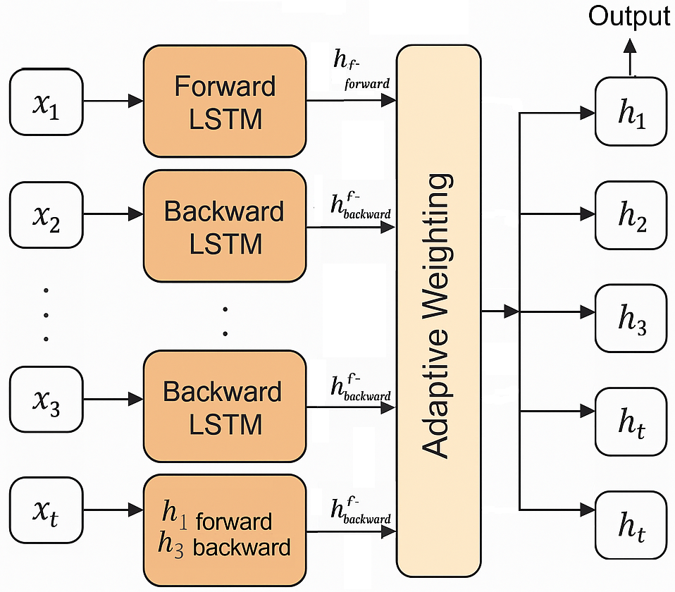
The equations presented indicate that adaptive weight based amplification is effectively carried out within the LSTM. Therefore, it proves instrumental in generating precise crop recommendation outcomes [27]. Figure 1 shows the general architecture of AWBiLSTM model.
The performance evaluation of the MSSA-AWBiLSTM method is carried out using Python 3.6.5 on a PC equipped with an i5-8600k processor, GeForce 1050Ti 4 GB GPU, 16 GB RAM, 250 GB SSD, and 1 TB HDD. The proposed MSSA-AWBiLSTM is compared with existing AWBiLSTM model to assess its effectiveness. Notably, the proposed MSSA-AWBiLSTM model surpasses existing classification algorithms [28, 29, 30, 18, 19] for crop recommendation across various performance metrics including recall, precision, accuracy, specificity, Precision Recall Curve (PR-Score), receiver operating characteristic (ROC-Score), F1-Score, Matthews correlation coefficient (MCC), R2-Score and execution time. These algorithms have previously demonstrated their performance in related literature. The comparison of performance evaluation metrics is presented in Table 1.
| Performance Metrics | Values |
|---|---|
| Accuracy | 98.72 |
| Precision | 98.81 |
| Recall | 98.54 |
| Specificity | 98.10 |
| PR-Score | 98.18 |
| ROC-Score | 98.49 |
| F1-Score | 98.48 |
| MCC | 97.63 |
Table 1 shows the crop recommendation results obtained from the MSSA-AWBiLSTM. Results demonstrate superior performance with an accuracy of 98.72%, precision of 98.81%, recall of 98.54%, specificity of 98.10%, PR-score of 98.18%, ROC-score of 98.49%, F1-score of 98.48%, and MCC of 97.63%.
Table 2 presents a comparative analysis of crop recommendation results achieved by the MSSA-AWBiLSTM model alongside existing models, including [12, 28, 29, 30, 19]. The crop recommendation outcomes of the MSSA-AWBiLSTM model are compared with those of existing models in terms of R2 score, as presented in Table 3. These values affirm the superior crop recommendation capabilities of the MSSA-AWBiLSTM model compared to other models.
| Methods | Accuracy | Precision | Recall |
|
||
|---|---|---|---|---|---|---|
| XAI-CROP | 95.12 | 95.62 | 95.78 | 95.86 | ||
|
92.68 | 90.88 | 91.98 | 91.79 | ||
|
98.72 | 98.81 | 98.54 | 98.48 | ||
| RFOERNN | 98.45 | 98.51 | 98.45 | 98.46 | ||
| MMML | 97.91 | 97.97 | 97.91 | 97.92 | ||
| NC-SAE | 94.64 | 94.06 | 94.78 | 95.49 | ||
|
91.73 | 91.13 | 92.42 | 93.80 | ||
| SVM | 89.49 | 88.17 | 88.70 | 88.46 | ||
| SSAE-CNN | 90.85 | 93.86 | 90.60 | 92.94 | ||
| PCA-CNN | 88.62 | 89.27 | 87.75 | 89.08 | ||
| DT | 85.07 | 84.73 | 85.91 | 85.39 |
| Methods | R2-Score |
|---|---|
| XAI-CROP | 94.15 |
| IDCSO-WLSTM | 92.54 |
| MSSA-AWBiLSTM | 99.14 |
| RFOERNN | 99.88 |
| MMML | 98.54 |
| SVR | 91.99 |
| KNN | 87.05 |
| MLR | 89.10 |
| ANN | 91.97 |
When the proposed method operates at a faster pace, it signifies an improvement in the system's efficiency. Both the proposed MSSA-AWBiLSTM algorithm and the current methods are utilized to compare their execution times as a measure of comparison. Remarkably, the MSSA-AWBiLSTM algorithm demonstrates shorter execution times when applied to the crop recommendation dataset. Table 4 provides a comparison between the existing and proposed systems based on Execution Time (in seconds).
| Methods | Execution time (sec) |
|---|---|
| XAI-CROP | 240.0554 |
| IDCSO-WLSTM | 241.0484 |
| MSSA-AWBiLSTM | 228.0112 |
| RFOERNN | 240.0529 |
| MMML | 242.0492 |
| SVR | 242.0532 |
| KNN | 241.0639 |
| MLR | 242.0677 |
| ANN | 242.0704 |
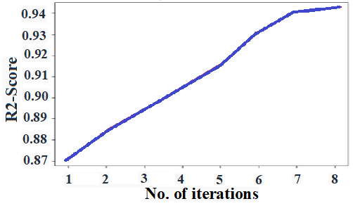
Figure 2 depicts the R2 convergence curve derived from the MSSA-AWBiLSTM model. This curve gives crucial information about the model's performance and capacity to simulate the dataset's intrinsic patterns and connections. The R2 convergence curve, which serves as an indicator of convergence during training, shows the R2 score on the y-axis against the number of iterations on the x-axis. The R2 score indicates how much of the target variable's variance is explained by the proposed model. A higher R2 value shows that the model is more aligned with the data and has enhanced prediction accuracy. Analysis of the R2 convergence curves allows researchers to gauge training dynamics, performance stability, convergence rate, and the potential for overfitting or underfitting.
Soil pH, nitrogen (N), phosphorus (P), potassium (K), organic carbon, temperature, rainfall, humidity, sunshine hours, soil type index, and area ID were among the important variables that were included in the multivariable analysis for crop recommendation. Principal component analysis (PCA) was performed to reduce dimensionality and maintain 95% of the variance using the top six principal components, while multiple linear regression (MLR) was utilized to evaluate the effect of these factors on crop yield. Additionally, the analysis used the variance inflation factor (VIF) to check for multicollinearity and the analysis of variance (ANOVA) to assess the significance of the grouped variables. The AWBiLSTM ensemble model was used to improve prediction after the MSSA selected features based on the PCA results. The main conclusion of the analysis were that temperature, rainfall, and soil pH all significantly affected crop yield (p < 0.01). Furthermore, when multivariable features were used instead of raw input data, AWBiLSTM performance increased.
Agriculture is the primary livelihood for farmers, making crop selection based on soil conditions crucial for maximizing yield. Data-driven recommendations using ML and IoT can significantly improve farmers' decision-making, reducing costs and enhancing precision in precision agriculture. This study presents a novel MSSA-AWBiLSTM method for crop recommendation and yield prediction, addressing the challenge of selecting the most suitable crop during the growing season. The model is fine-tuned using region-specific data and validated for different soil types.
The MSSA algorithm selects key features from the dataset, while AWBiLSTM predicts and recommends crops using an LSTM network ensemble with adaptive weighting. Experimental results show that MSSA-AWBiLSTM outperforms other methods, achieving a 98.72% improvement in crop prediction accuracy and a higher R2 value by optimally selecting climate parameters.
While the MSSA-AWBiLSTM method improves crop prediction, it may not perform well with weed species detection. Future work will focus on expanding the dataset with more variables, integrating yield prediction, and incorporating market factors, such as post-harvest storage and profitability, to further enhance and validate the proposed model's applicability.
The MSSA-AWBiLSTM approach has drawbacks despite its great accuracy. It might have trouble with tasks that need for multiple kinds of data, including inputs based on images, like weed species detection. Additionally, the model's scalability may be constrained by the availability and quality of region-specific data. Furthermore, outside variables like insect outbreaks and market dynamics are not taken into account. Future studies will concentrate on adding more economic and environmental factors, broadening the dataset to encompass a variety of crop and soil types, and improving the model to facilitate post-harvest decision-making, storage planning, and profitability forecasting for more useful implementation.
IECE Transactions on Swarm and Evolutionary Learning
ISSN: request pending (Online) | ISSN: request pending (Print)
Email: [email protected]

Portico
All published articles are preserved here permanently:
https://www.portico.org/publishers/iece/