Enhanced Differential Evolution: Multi-Strategy Approach with Neighborhood-Based Selection

Elivier Reyes-Davila; Eduardo H. Haro; Angel Casas-Ordaz; Diego Oliva; Saúl Zapotecas-Martínez; Mohammed El-Abd

doi:10.62762/TSEL.2025.182681

Abstract

The Differential Evolution (DE) has stood as a cornerstone of Evolutionary Computation (EC), inspiring numerous approaches. Despite its foundational role, the selection stage of DE has received little attention, with only 2% of documented modifications in the literature on this aspect. Recent research has underscored the potential for significant algorithmic improvement through thoughtful modifications to this critical stage, particularly in accelerating the exploitation phase. This study introduces a novel EC strategy rooted in DE principles. To enhance algorithmic exploration, a systematic decision-making process regarding function evaluations is employed to select between two of the most prevalent mutations in the field. Similarly, a new selection operator is introduced to augment the exploitation phase by comparing each individual with its respective 25% neighborhood population. The proposed algorithm, Differential Evolution with Selection by Neighborhood (DESN), undergoes comprehensive evaluation against eight classical and recent approaches, leveraging the CEC-2017 set of benchmark functions.

Keywords

differential evolution

mutation operator

selection mechanisms

1. Introduction

Differential Evolution (DE) stands as one of the most esteemed algorithms within Evolutionary Computation (EC), initially introduced by Storn et al. [1]. Since its inception in 1995, DE has found wide-ranging applications in scientific and engineering domains [2], inspiring numerous EC approaches that have become pivotal benchmarks in the literature [3]. In the specialized literature, most approaches have been derived from schemes involving tailored modifications to DE's key stages, such as initialization, mutation, crossover, and selection mechanisms. Notably, mutation and crossover operators, along with the tuning of their parameters, have been the focal points of extensive research efforts.

In the last few years, a significant number of variations of the DE algorithm have been developed that have proven to be both novel and noteworthy [4]. These variations have demonstrated the algorithm's capacity for enhancement in varied ways, underscoring its adaptability and flexibility. This flexibility has enabled the DE to align with a substantial body of related research, making it challenging to comprehensively survey all relevant works in a single compendium, as evidenced by Pant et al. [5]. A notable example is the Chaotic Opposition-based-learning Differential Evolution (CODE) algorithm, which proposes the implementation of chaotic maps and an opposition-based learning strategy to develop a novel variant of DE featuring a modified initialization scheme [6]. Additionally, a proposal known as Dynamic Combination Differential Evolution (DCDE) [7] has emerged, which involves a variant of the mutation operator based on the dynamic combination and a two-level parameter regulation strategy. Additionally, the Adaptive Differential Evolution With Optional External Archive (JADE) algorithm [8] is noteworthy for implementing a novel mutation strategy with an optional external file and adaptively updating the control parameters.

Various proposals regarding mutation operators have surfaced in the literature, such as the triangular mutation [9] and the hemostasis-based mutation [10]. On the other hand, crossover operators have been presented, such as the parent-centered crossover [11] and the multiple exponential crossover [12]. However, the literature on selection stage modifications remains relatively sparse, with fewer related works emerging over the past decade. One prominent investigation in this domain is the new selection operator algorithm (NSO) proposed by Zeng et al. [13]. However, in general terms, investigations on selection mechanisms for DE represent a small fraction, approximately 2%, of the modifications reported in the specialized literature [5]. Conversely, advancements in evolutionary computation and machine learning have demonstrated substantial progress [14, 15, 16]. The development of these algorithms has created a range of possibilities for modifications, which can be implemented in specialized areas [17, 18].

To provide novel insights into the DE selection stage, this paper introduces Differential Evolution with Selection by Neighborhood (DESN), a new evolutionary algorithm with an improved selection mechanism. DESN employs a decision variable based on current function access to choose between two classical mutation strategies: DE/rand/2 and DE/best/1. Additionally, it features a selection stage where the current trial vector is compared against its individual and its neighborhood, which constitutes approximately 25% of the population. These modifications markedly enhance the algorithm's performance, improving exploration and exploitation phases compared to the original DE.

DESN's efficacy is evaluated on the benchmark functions of the 2017 Congress on Evolutionary Computation (CEC) against eight other established evolutionary and meta-heuristic algorithms. Computational experiments demonstrate DESN's superior performance in exploration and exploitation, with the Friedman test confirming its superiority. Furthermore, a Big O analysis affirms DESN's competitive computational cost, establishing it as a promising algorithm for future applications.

The paper is structured as follows: Section 2 provides a general background to understand the presented work, Section 3 details the proposed DESN, Section 4 presents computational and statistical results, and Section 5 discusses the conclusions.

2. General Background

2.1 Differential evolution algorithm

The DE algorithm, similar to numerous optimization algorithms, was conceived to address real-world problems[19]. Its fundamental algorithmic structure encompasses four phases: initialization, mutation, crossover, and selection. Notably, it operates as a population-based stochastic search method, with its efficacy being contingent upon the mutation strategy, crossover strategy, and control parameters such as population size ( $N p$ ), crossover rate ( $C r$ ), and scale factor ( $F$ ). To illustrate the algorithm's framework, each phase is delineated as follows.

2.1.1 Initialization

The algorithm begins with initialization, a crucial step where the search space limits for the optimization problem are defined. Each individual solution within the population is represented as a $d$ -dimentional vector during the $g$ -th generation, denoted as:

x^{g}_{i}={\bigl{\{}x^{g}_{i,1},x^{g}_{i,2}\ldots,x^{g}_{i,d}\bigr{\}}},\ i=1,% \ldots,Np

where $N p$ signifies the population size, $g$ denotes the generation index, and $d$ represents the dimensionality of the problem.

The individual vectors are generated according to the equation:

x^{0}_{i,d}={x_{min,d}+rand(0,1)*(x_{max,d}-x_{min,d})}

where $rand(0,1)$ symbolizes a uniformly distributed random variable ranging from 0 to 1. $x_{min}$ and $x_{max}$ denote the lower and upper bounds for each dimension of the search space, defined as:

x_{min}=(x_{min,1},\ldots,x_{min,d})

x_{max}=(x_{max,1},\ldots,x_{max,d})

2.1.2 Mutation

Following initialization, the DE algorithm employs a random perturbation process on each candidate solution. This process reshuffles the elements of the population to create a modified version of each individual, resulting in the creation of mutant vectors $v^{g}_{i}$ . The widely adopted mutation strategy in DE, known as DE/rand/1, is defined by the equation:

v^{g+1}_{i}=x^{g}_{r3}+F(x^{g}_{r1}-x^{g}_{r2})

where $x_{r1},x_{r2},x_{r3}$ are randomly selected population vectors considering that $r1\neq r2\neq r3\neq i$ (index of the target vector), and $F$ is the scale factor that is a fixed value in the range of $[0,2]$ .

2.1.3 Crossover

To complement mutation, the crossover strategy enhances population diversity. Governed by the crossover probability ( $C r$ ), a constant value within the range $[0,1]$ , this strategy necessitates user-defined determination. Generating a new vector, termed the trial vector $u_{i}^{g}$ , involves a crossover between the target vector $x_{i,d}^{g}$ and the mutant vector $v_{i,d}^{g}$ as follows:

u^{g+1}_{i}=u^{g}_{d}\begin{cases}v^{g}_{i,d}&\text{if }d=d_{rand}\text{ or }% rand(0,1)\leq Cr\\ x^{g}_{i,d}&\text{otherwise}\end{cases}

where $d_{rand}$ denotes a randomly chosen index from $\{1,2,\ldots,d\}$ , ensuring $u^{g}_{i}$ encompasses at least one parameter of the mutant vector $v^{g}_{i}$ .

2.1.4 Selection

The selection process in DE determines the survival of target or trial solutions in the subsequent generation based on their fitness values. The vector with the fittest values progresses to the next generation's population. This operation is described as:

x^{g+1}_{i}=\begin{cases}u^{g}_{i,j}&\text{if}\ f(u^{g+1}_{i})\leq f(x^{g}_{i}% ),\\ x^{g}_{i,j}&\text{otherwise},\end{cases}

Once the new population is established, the mutation, crossover, and selection processes are iterated until the optimum solution is found or a specified termination criterion is met.

3. Proposed Approach

The proposed DESN introduces a series of three targeted modifications to enhance the efficiency and efficacy of the standard DE algorithm. Firstly, an adjustment is made to the mutation stage, where traditional DE algorithms typically employ a predefined mutation strategy. In the proposed DESN, this stage undergoes refinement to accommodate a more nuanced approach, which aims to foster greater diversity and exploration within the population. Secondly, the selection stage, which governs the retention and propagation of candidate solutions, undergoes scrutiny and optimization in the proposed DESN. The selection process is fine-tuned through strategic adjustments and enhancements to identify better and prioritize promising candidate solutions, thereby enhancing the algorithm's ability to converge toward optimal or near-optimal solutions. Thirdly, DESN incorporates a novel control parameter adaptation scheme, leveraging the iterative process's dynamics to dynamically adjust key parameters such as scaling factor ( $F$ ) and crossover rate ( $C r$ ). By monitoring the iterative process for signs of stagnation or diminishing returns, DESN adapts these parameters dynamically, thereby promoting sustained exploration and exploitation throughout the optimization process. Collectively, these above modifications synergistically contribute to the overall effectiveness and versatility of DESN, enabling it to tackle a wider range of optimization problems with improved efficiency and robustness compared to traditional DE algorithms.

The DE/rand/1 mutation, a cornerstone of the canonical differential evolution algorithm, is renowned for its adept exploration capabilities while exhibiting limitations in effectively exploiting promising regions. Conversely, though proficient in exploitation, the DE/best/1 mutation is prone to stagnation, particularly in multimodal problems. Recognizing the inherent trade-offs within these mutation operators, it becomes evident that no single strategy satisfactorily addresses the diverse challenges encountered across optimization landscapes.

In response to this realization, a strategic unification of mutation strategies is proposed. By leveraging the strengths of both DE/rand/2 and DE/best/1 strategies, as shown in Equation (1) and Equation (2) respectively. The aim is to synthesize a hybrid approach that capitalizes on the complementary advantages of each strategy. This unification approach seeks to balance the exploration- exploitation trade-off inherent in optimization processes, thereby enhancing the algorithm's ability to navigate complex and dynamic search spaces.

v^{g+1}_{i}=x^{g}_{r5}+F(x^{g}_{r1}-x^{g}_{r2})+F(x^{g}_{r3}-x^{g}_{r4})

v^{g+1}_{i}=x^{g}_{best}+F(x^{g}_{r1}-x^{g}_{r2})

By integrating diverse mutation strategies, the proposed approach endeavors to harness the best capabilities of each strategy while mitigating their limitations. Through this synthesis, the algorithm aims to achieve a more robust and adaptive optimization framework capable of addressing a broader spectrum of optimization challenges with heightened efficacy and efficiency.

The classical DE/rand/1 mutation, renowned for its prowess in exploration, encounters challenges in fully exploiting promising regions within the search space. On the contrary, the DE/best/1 mutation excels in exploitation but often grapples with stagnation, particularly in complex multimodal problems. Acknowledging the inherent constraints of individual mutation operators, a compelling impetus arises to harness the collective strengths of the DE/rand/2 and DE/best/1 strategies.

Through a strategic integration of these mutation schemes, as described in Equation (1) and Equation (2), respectively, a balanced and synergistic approach to the search process emerges. By leveraging the exploratory capabilities of DE/rand/2 alongside the exploitation-enhancing features of DE/best/1, the consolidated strategy seeks to mitigate the shortcomings of each method.

This unification aims to foster a more robust and adaptive optimization framework capable of navigating the intricacies of diverse optimization landscapes with heightened efficacy and resilience. By orchestrating a harmonious interplay between exploration and exploitation, the proposed approach strives to transcend the limitations inherent in traditional mutation strategies, thereby advancing the frontiers of evolutionary optimization methodologies.

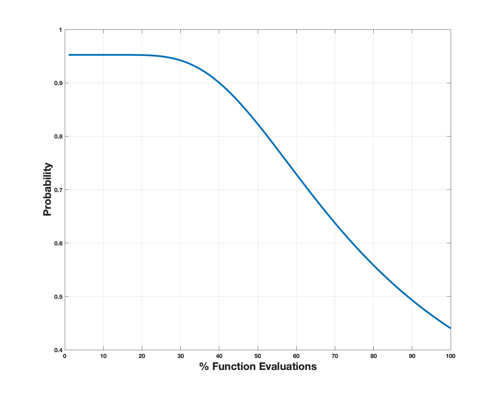
Determining which strategy to employ relies on the sigmoid function depicted in Equation (3). Essentially, this function governs the likelihood of utilizing the DE/rand2 mutation.

Pmut=\frac{1}{1+e^{1.05-(FE_{max}/FE)^{2}}}

From Equation (3) $F E$ corresponds to the number of function evaluations. Figure 1 visually represents this function. Observation of the plot reveals that within the initial 25 % of function evaluations, the probability of selecting the exploration-oriented mutation stands at approximately 0.95. Subsequently, in the middle phase of the search process, this probability declines to around 0.82. Towards the concluding stages, it further diminishes to approximately 0.45, affording the algorithm greater opportunities to exploit the present region. As illustrated in Figure 1, this approach fosters a balanced integration of the diverse mutation options, meticulously calibrated in a strategic manner. The interchangeable behavior between the different mutations, with a variable probability percentage guided by the sigmoid function, generates a superior combination of exploration and exploitation, thereby enhancing the algorithm's performance.

Figure 1 Indicator of the percentage of probability for the chosen mutation.

Conversely, many researchers concur that no single set of control parameters ensures optimal performance for the Differential Evolution (DE) algorithm across diverse problem domains [21]. Consequently, the DE algorithm must be able to adjust the influence of both mutation and crossover operators while generating trial solutions. One proposed solution involves the incorporation of a stagnation counter ( $s$ ): each time a trial solution fails to improve upon the best solution, this counter increments by one unit. If it surpasses the population size, the values of $F$ and $C R$ are randomly reset within the range of [0,1].

Furthermore, in the selection stage, each trial vector is evaluated against $n$ neighboring solutions of the target vector. Extensive experimentation revealed that setting $n$ to 25% of the population size yields optimal results. For instance, in a population comprising 100 solutions where the target vector is the tenth element, the trial vector is compared with solutions indexed from 10 to 35. Subsequently, the worst-performing solution among them is replaced by the trial vector. This mechanism enhances the likelihood of integrating the trial vector into the population, thereby minimizing redundant function evaluations. This behavior is reflected in Algorithm 1. As can be seen, the initial behavior of the choice of mutation type is determined by the $P m u t$ value (within lines 6-11). Subsequently, the crossover operator is carried out. Following this, selection based on neighbors is implemented. Subsequent to this, the behavior of taking into account 25% of the population is initiated, culminating in the selection of the optimal solution (lines 16-28). Finally, the stagnation value is determined to ascertain whether the values of $F$ and $C r$ will undergo random modification.

Algorithm 1 DE with selection by neighborhood

Initialize parameters $C r, F$ , $N p$ , iteration and stagnation counters $g\leftarrow 0$ , $s\leftarrow 0$ . ;
Initialize population with Equation (1) ;
Determine the size of the neighborhood $n\leftarrow(Np*0.25)$ ;
while stop condition not met do
for $i=1:Np$ do
Determine $P m u t$ $\triangleright$ Equation (3) ;
if $rand\leq Pmut$ then
$v^{g}_{i}$ $\leftarrow$ $DE/rand/2$ $\triangleright$ Equation (1);
else
$v^{g}_{i}$ $\leftarrow$ $DE/best/1$ $\triangleright$ Equation (2);
end if
$u^{g}_{i}$ $\leftarrow$ crossover $\triangleright$ Equation (6) ;
if $i>0.75*Np$ then
$n=n-1$ ;
end if
for $k=0:n-1$ do
if $f(u^{g}_{i})\leq f(x^{g}_{i+k})$ then
${x^{g+1}_{i}}\leftarrow u^{g}_{i}$ ;
if $f(u^{g}_{i})\leq f(x_{best})$ then
${x_{best}}\leftarrow u^{g}_{i}$ ;
$s=0$ ;
else
$s=s+1$
end if
Break
else
${x^{g+1}_{i}}\leftarrow x^{g}_{i}$ ;
end if
end for
if $s>Np$ then
$F=rand$ ;
$Cr=rand$ ;
end if
end for
$g\leftarrow g+1$ ;
end while

4. Experimental Study and Analysis of Results

This section presents the outcomes derived from comparative computational experiments. All algorithms were executed under uniform conditions: 30 dimensions, 50,000 function evaluations, and 35 independent runs conducted in the MATLAB environment on a Notebook (2.7 GHz processor, 8 GB RAM) running Windows 10 OS. The proposed DESN is assessed using the 30 benchmark functions from CEC-2017, categorized into unimodal, multimodal, hybrid, and compositional functions [20]. Moreover, DESN is computationally contrasted against eight distinct algorithms, including the original DE [1] and Covariance Matrix Adaptation with Evolution Strategies (CMAES) [22]. Additionally, three contemporary meta-heuristic algorithms, namely the Reptile Search Algorithm (RSA) [23], the Runge Kutta Optimizer (RUN) [24], and the Nutcracker Optimization Algorithm (NOA) [25], are included. Finally, three classical algorithms from the evolutionary literature, comprising Simulated Annealing (SA) [26], the well-established Particle Swarm Optimization algorithm (PSO) [27], and the original Genetic Algorithm (GA) [28] are considered. Detailed parameters of these algorithms are provided in Table 1.

Table 1 Specific parameters of the algorithms.

Parameters	Symbol	Value	Algorithm
Scaling factor	$F$	0.8	DESN / DE
Crossover rate	$C r$	0.2	DESN / DE
Neighborhood rate	$N v$	0.25	DESN
Constant of change	$\alpha$	0.1	RSA
Step size	$\beta$	0.005	RSA
Step rate	$\alpha_{\mu}$	8	CMAES
Attempts rate	$\alpha$	100	NOA
Change rate	$P a$	0.0001	NOA
Exploration rate	$P r$	0.0001	NOA
Increase rate	$\beta$	0.98	SA
Crossing rate	$R c$	0.8	GA
Mutation rate	$R m$	0.2	GA

Table 2 Statistical results for benchmark functions in 30 dimensions (Part 1).

Function		Algorithms
No	Metric	DESN	DE	CMAES	RSA	RUN	NOA	SA	PSO	GA
F1	Average	1.94E+05	3.36E+08	1.54E+09	4.10E+10	1.98E+10	1.01E+07	1.19E+11	3.31E+10	4.03E+10
	STD	5.09E+04	8.29E+07	1.37E+10	1.42E+10	1.39E+09	5.03E+06	6.13E-05	8.59E+09	1.41E+10
	Rank Avg	1	3	4	8	5	2	9	6	7
F2	Average	5.92E+21	5.89E+46	-3.54E+270	1.50E+54	2.17E+31	7.89E+28	2.35E+47	3.82E+39	9.35E+54
	STD	2.35E+22	4.99E+47	Inf	1.50E+55	1.74E+32	4.99E+29	4.08E+31	2.96E+40	9.32E+56
	Rank Avg	2	6	1	8	4	3	7	5	9
F3	Average	7.02E+04	7.86E+05	1.55E+08	1.99E+10	1.57E+05	1.02E+05	1.49E+05	2.56E+05	1.87E+10
	STD	3.35E+04	7.30E+05	1.49E+10	1.99E+11	6.56E+04	6.98E+04	0.00E+00	4.64E+05	3.75E+12
	Rank Avg	1	6	7	9	4	2	3	5	8
F4	Average	4.87E+02	1.04E+03	1.16E+03	9.50E+03	2.03E+03	5.43E+02	2.62E+04	3.53E+03	1.17E+04
	STD	3.63E-02	2.42E+02	7.92E+03	1.80E+04	1.67E+02	1.90E+01	1.10E-11	1.35E+03	5.71E+03
	Rank Avg	1	3	4	7	5	2	9	6	8
F5	Average	6.06E+02	8.01E+02	6.92E+02	9.67E+02	8.61E+02	7.33E+02	1.19E+03	9.02E+02	9.54E+02
	STD	1.02E+01	3.16E+01	5.50E+01	1.25E+02	2.05E+01	3.44E+01	6.86E-13	3.13E+01	1.68E+01
	Rank Avg	1	4	2	8	5	3	9	6	7
F6	Average	6.01E+02	6.15E+02	6.05E+02	6.88E+02	6.60E+02	6.05E+02	7.45E+02	6.70E+02	6.90E+02
	STD	9.60E-02	2.13E+00	1.84E+01	1.04E+01	3.52E+00	1.06E+00	1.14E-13	7.30E+00	1.79E+01
	Rank Avg	1	3	2	6	4	2	8	5	7
F7	Average	9.20E+02	1.04E+03	9.44E+02	1.44E+03	1.31E+03	9.78E+02	3.47E+03	2.26E+03	2.00E+03
	STD	2.12E+01	3.61E+01	2.30E+02	3.04E+02	3.52E+01	2.79E+01	1.83E-12	3.55E+02	1.31E+02
	Rank Avg	1	4	2	6	5	3	9	8	7
F8	Average	8.47E+02	1.09E+03	9.85E+02	1.16E+03	1.13E+03	1.01E+03	1.31E+03	1.19E+03	1.22E+03
	STD	4.18E-03	3.23E+01	4.38E+01	6.79E+01	2.16E+01	2.75E+01	4.57E-13	3.21E+01	2.35E+01
	Rank Avg	1	4	2	6	5	3	9	7	8
F9	Average	9.05E+02	1.49E+04	1.40E+03	1.50E+04	1.01E+04	1.11E+03	3.09E+04	1.44E+04	1.49E+04
	STD	6.60E-01	4.37E+03	3.60E+03	8.58E+03	1.14E+03	8.61E+01	7.31E-12	2.17E+03	1.48E+03
	Rank Avg	1	6	3	7	4	2	8	5	6
F10	Average	4.23E+03	9.10E+03	8.33E+03	8.50E+03	6.91E+03	9.24E+03	1.07E+04	8.08E+03	8.54E+03
	STD	1.30E-01	5.87E+02	3.17E+02	6.85E+02	1.09E+02	5.47E+02	7.31E-12	4.77E+02	6.08E+02
	Rank Avg	1	7	4	5	2	8	9	3	6

Tables 2, 3 and 4 exhibit the statistical outcomes derived from 35 runs performed for each algorithm. For comparison, key metrics were computed for each method, including Average, standard deviation (STD), and a ranking based on the Average of the 35 runs (Rank Avg). The stop criteria for all algorithms is the maximum number of function evaluations. The tables are organized as follows: Table 2 displays the results of the unimodal and multimodal functions, Table 3 showcases the results for hybrid functions, and Table 4 presents the results for composition functions. To enhance clarity, exceptional values are highlighted in bold for easier identification.

(a) Function 1

(b) Function 10

Figure 2 Convergences of unimodal and multimodal functions.

The objective of conducting experimental tests on this benchmark, which comprises different categories of functions, is to validate the effectiveness and robustness of the algorithms in various scenarios. In the context of unimodal functions, these functions can be characterized as those that possess a global maximum (also known as a peak) or a global minimum (trough) in the interval $[a,b]$ . These functions are designed to assess the exploitability of the algorithms, given the presence of a single optimum. Conversely, multimodal functions contain more than one "mode" or optimum, which often creates difficulties for any optimization algorithm since there are many attractors that the algorithm can target. Consequently, these functions necessitate a greater emphasis on exploratory behavior to circumvent the stagnation at the local optima. On the other hand, there are composite functions. This type of function consists of several unimodal and multimodal functions, increasing the search process's difficulty. The idea of testing algorithms on this type of function is to test the algorithm's performance in finding randomly located global optima while avoiding falling into several deep local optima scattered in the same random way as the global optima. Finally, we have the hybrid or shifted functions. These functions are designed to move the global optimum to a different location than it originally had in some of the previous unimodal and multimodal functions. This tests whether the algorithms have the well-documented design flaw whereby some metaheuristic algorithms seem to perform better only when the optimization problem has the global optimum at position zero.

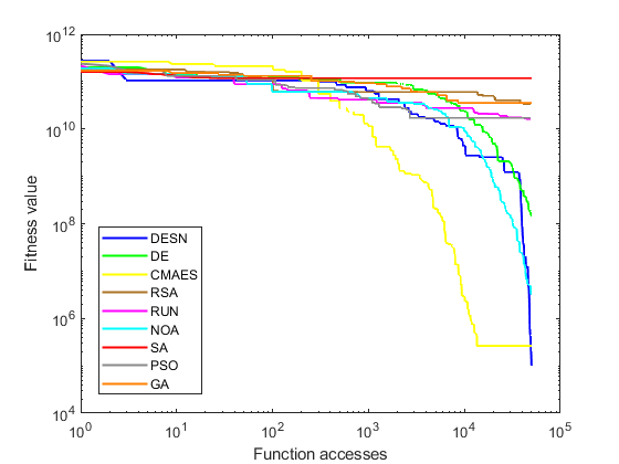
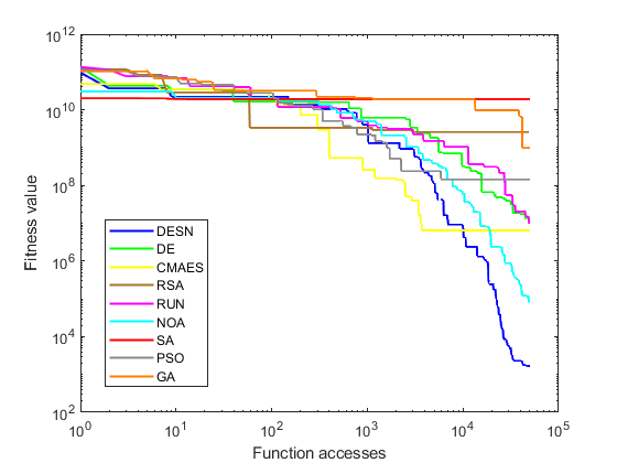
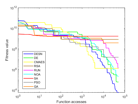
Table 2 highlights that the proposed DESN algorithm achieves superior results compared to other algorithms. Remarkably, DESN performed notably better for problems F1 and F3- F10. SA showed similar values, albeit solely in standard deviation. It is worth noticing that F2 was excluded due to its unstable behaviors [20]. Building upon the outcomes in Table 2, Figure 2 provides a graphical representation of convergence results for unimodal and multimodal functions. These convergences are based on the best metric results of the respective algorithms. Figure 2(a) illustrates a sample of the unimodal function F1, where DESN outperforms other algorithms, with CMAES and NOA displaying competitive potential but getting stuck in local optima. Conversely, Figure 2(b) demonstrates a sample of the multimodal function (F10), where DESN again exhibits superior performance compared to other approaches. Moreover, no algorithm emerges victorious in multimodal functions or competes effectively with DESN. The behavior of the DESN algorithm indicates its capacity to identify global optima within this particular function type. This finding underscores the algorithm's versatility in this particular class of functions.

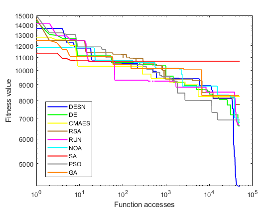
Table 3 demonstrates analogous patterns to the preceding tables. Across all instances of the DESN algorithm, favorable outcomes are observed, except for the standard deviation of the SA, where results deviate consistently. As indicated by the data in Table 3, Figure 3 showcases convergence samples of hybrid functions (F12 and F13). These convergences correspond to the best metric results, shown in Figure 2. Specifically, F12 and F13 are chosen for their notable disparities. Both Figure 3(a) and Figure 3(b) reveal consistent performance by the DESN, surpassing other algorithms, with CMAES and NOA emerging as the sole competitive alternatives.

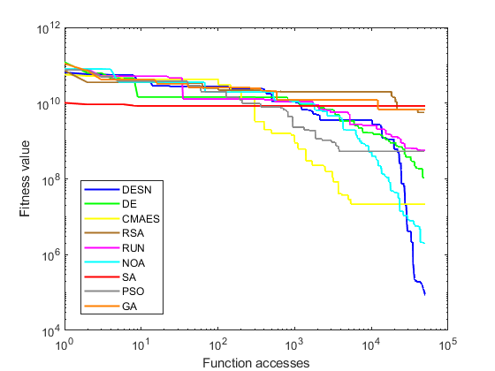
Table 4 demonstrates that, overall, the DESN algorithm performs the best across most cases, except for function 26, where the NOA algorithm shows superior performance. Further exploring convergence, Figure 4 provides a visual analysis of convergence for two samples from the composition functions, corresponding to the results outlined in Table 4. It is important to note that the convergence analysis presented relies on the best metric results, as indicated by Figure 2 and Figure 3. It is widely acknowledged that composition functions are inherently more challenging compared to other benchmark functions [29]. Thus, the performances depicted in Figure 4(a) and Figure 4(b) align with those reported in Table 4. Both samples illustrate DESN outperforming other algorithms, albeit with marginal differences. Notably, no algorithm surpasses DESN, while CMAES and NOA emerge as the most competitive algorithms, with DE being the most competitive approach.

Table 3 Statistical results for benchmark functions in 30 dimensions (Part 2).

Function		Algorithms
No	Metric	DESN	DE	CMAES	RSA	RUN	NOA	SA	PSO	GA
F11	Average	1.14E+03	1.50E+04	3.69E+05	4.63E+07	3.31E+03	1.48E+03	1.96E+04	9.72E+03	9.69E+04
	STD	2.06E+00	1.04E+04	2.73E+07	4.62E+08	9.28E+02	1.44E+02	7.31E-12	3.01E+03	1.40E+07
	Rank Avg	1	5	8	9	3	2	6	4	7
F12	Average	1.16E+05	6.55E+08	2.22E+08	9.27E+09	7.19E+08	1.34E+07	8.45E+09	2.90E+09	8.23E+09
	STD	1.11E+04	2.49E+08	2.33E+09	6.48E+09	1.31E+08	8.43E+06	1.92E-06	1.20E+09	2.94E+09
	Rank Avg	1	4	3	9	5	2	8	6	7
F13	Average	1.71E+03	7.61E+07	1.27E+08	7.14E+09	7.50E+07	1.13E+06	1.92E+10	1.94E+09	1.07E+10
	STD	1.18E+01	5.42E+07	1.58E+09	1.12E+10	4.99E+07	1.04E+06	1.15E-05	1.11E+09	6.34E+09
	Rank Avg	1	4	5	7	3	2	9	6	8
F14	Average	1.49E+03	1.45E+07	6.60E+05	2.84E+07	2.39E+04	6.03E+03	8.01E+05	4.80E+06	9.61E+06
	STD	1.15E+01	2.11E+07	8.79E+06	2.45E+08	2.06E+04	1.18E+04	1.17E-10	4.25E+06	1.77E+07
	Rank Avg	1	8	4	9	3	2	5	6	7
F15	Average	1.67E+03	2.17E+07	3.24E+07	4.39E+08	7.18E+05	9.81E+04	1.03E+09	5.98E+08	5.37E+08
	STD	6.23E+00	2.23E+07	5.26E+08	2.31E+09	1.62E+06	2.08E+05	0.00E+00	4.32E+08	5.09E+08
	Rank Avg	1	4	5	6	3	2	9	8	7
F16	Average	1.95E+03	4.39E+03	3.25E+03	7.78E+03	3.58E+03	3.86E+03	9.44E+03	4.28E+03	5.01E+03
	STD	1.71E-01	4.13E+02	1.58E+03	1.11E+04	2.17E+02	3.81E+02	1.83E-12	4.35E+02	5.53E+02
	Rank Avg	1	6	2	8	3	4	9	5	7
F17	Average	1.89E+03	3.01E+03	3.02E+03	1.59E+04	2.13E+03	2.53E+03	5.84E+04	3.39E+03	4.13E+03
	STD	1.31E+01	2.55E+02	4.78E+04	1.10E+05	6.19E+01	2.52E+02	1.46E-11	2.87E+02	6.37E+04
	Rank Avg	1	4	5	8	2	3	9	6	7
F18	Average	1.07E+05	6.32E+07	3.68E+06	1.86E+08	6.52E+05	1.12E+06	3.63E+07	1.05E+07	1.68E+07
	STD	2.58E+04	6.04E+07	2.50E+07	3.03E+08	5.42E+05	1.48E+06	7.49E-09	1.10E+07	1.58E+08
	Rank Avg	1	8	4	9	2	3	7	5	6
F19	Average	2.01E+03	2.24E+07	7.67E+07	8.41E+08	8.85E+05	1.94E+05	8.37E+09	8.22E+08	2.99E+08
	STD	1.11E+01	1.32E+08	1.29E+09	3.55E+09	1.32E+06	4.38E+05	1.92E-06	5.17E+08	4.04E+08
	Rank Avg	1	4	5	8	3	2	9	7	6
F20	Average	2.06E+03	3.15E+03	2.64E+03	3.31E+03	2.28E+03	2.91E+03	3.77E+03	2.83E+03	2.93E+03
	STD	2.16E-01	2.19E+02	1.91E+02	2.67E+02	3.45E+01	3.01E+02	1.37E-12	2.13E+02	3.62E+02
	Rank Avg	1	7	3	8	2	5	9	4	6

(a) Function 12

(b) Function 13

Figure 3 Convergences of hybrid functions.

Table 4 Statistical results for benchmark functions in 30 dimensions (Part 3).

Function		Algorithms
No	Metric	DESN	DE	CMAES	RSA	RUN	NOA	SA	PSO	GA
F21	Average	2.35E+03	2.60E+03	2.50E+03	2.69E+03	2.64E+03	2.53E+03	2.88E+03	2.68E+03	2.75E+03
	STD	6.98E-02	3.45E+01	4.95E+01	1.17E+02	2.00E+01	2.93E+01	1.37E-12	2.66E+01	2.18E+01
	Rank Avg	1	4	2	7	5	3	9	6	8
F22	Average	2.31E+03	1.05E+04	9.67E+03	8.06E+03	4.99E+03	2.33E+03	1.15E+04	6.00E+03	7.05E+03
	STD	7.65E-01	6.85E+02	4.25E+02	6.91E+02	1.56E+02	2.78E+00	0.00E+00	8.72E+02	1.14E+03
	Rank Avg	1	8	7	6	3	2	9	4	5
F23	Average	2.67E+03	3.00E+03	2.84E+03	3.51E+03	2.99E+03	2.89E+03	3.65E+03	3.00E+03	3.31E+03
	STD	1.61E-01	3.81E+01	8.42E+01	3.00E+02	2.27E+01	2.91E+01	1.83E-12	1.99E+01	8.65E+01
	Rank Avg	1	5	2	7	4	3	8	5	6
F24	Average	2.87E+03	3.20E+03	3.02E+03	3.57E+03	3.21E+03	3.05E+03	4.37E+03	3.13E+03	3.44E+03
	STD	5.13E-01	3.88E+01	1.44E+02	2.03E+02	2.70E+01	2.99E+01	9.14E-13	1.66E+01	1.13E+02
	Rank Avg	1	5	2	8	6	3	9	4	7
F25	Average	2.89E+03	3.19E+03	3.04E+03	4.50E+03	3.68E+03	2.91E+03	2.11E+04	5.81E+03	1.04E+04
	STD	4.22E-02	1.10E+02	1.43E+03	1.37E+03	7.46E+01	7.35E+00	3.66E-12	1.25E+03	1.89E+03
	Rank Avg	1	4	3	6	5	2	9	7	8
F26	Average	4.43E+03	6.38E+03	5.22E+03	1.04E+04	7.91E+03	3.61E+03	1.31E+04	7.47E+03	1.06E+04
	STD	4.24E+01	3.18E+02	1.08E+03	3.56E+03	2.40E+02	1.04E+03	0.00E+00	5.72E+02	1.11E+03
	Rank Avg	2	4	3	7	6	1	9	5	8
F27	Average	3.20E+03	3.20E+03	3.23E+03	3.91E+03	3.37E+03	3.29E+03	4.69E+03	3.27E+03	3.92E+03
	STD	3.80E-01	1.05E-04	3.40E+02	6.13E+02	1.43E+01	2.35E+01	1.83E-12	1.45E+01	2.26E+02
	Rank Avg	1	1	2	6	5	4	8	3	7
F28	Average	3.22E+03	3.30E+03	3.38E+03	6.27E+03	4.22E+03	3.24E+03	1.42E+04	4.46E+03	6.50E+03
	STD	4.68E-01	5.07E-02	8.43E+02	4.07E+03	1.24E+02	2.51E+01	0.00E+00	3.86E+02	5.66E+02
	Rank Avg	1	3	4	7	5	2	9	6	8
F29	Average	3.48E+03	5.22E+03	6.91E+03	1.59E+06	4.26E+03	4.98E+03	9.06E+03	5.00E+03	6.45E+03
	STD	1.82E+00	3.98E+02	1.57E+05	1.59E+07	8.89E+01	3.20E+02	5.48E-12	2.60E+02	1.82E+04
	Rank Avg	1	5	7	9	2	3	8	4	6
F30	Average	5.98E+03	1.05E+07	6.21E+07	1.49E+09	1.94E+07	3.21E+06	1.70E+09	3.63E+08	5.36E+08
	STD	5.19E+01	1.25E+07	9.65E+08	1.44E+09	1.58E+07	2.77E+06	0.00E+00	1.73E+08	3.74E+08
	Rank Avg	1	3	5	8	4	2	9	6	7

(a) Function 23

(b) Function 30

Figure 4 Convergences of composition functions.

Alternatively, resorting to statistical analysis and non-parametric tests becomes necessary when standard performance metrics fail to comprehensively compare algorithms. In such cases, well-established non-parametric models can be utilized to analyze and rank meta-heuristic algorithms [30]. The Friedman test, also known as Friedman's two-way ANOVA, is a prominent non-parametric test widely employed for analyzing differences among more than two related samples [31, 32]. Table 5 displays the Average Rank computed using the Friedman test for all algorithms under comparison. As shown in Table 5, the DESN proposal exhibited the highest rank among the algorithms considered. Moreover, the $p$ -value signifies significant differences among the assessed algorithms.

On the other hand, in these types of methods it is quite important to determine its computational consumption. Usually, comparisons of processing time tend to be considered through graphical schemes like boxplots [34]. Nonetheless, different studies have demonstrated the null-reliability of said approaches since the computational requirements of an algorithm change according to many aspects like the processor or other specifications [35, 33]. Hence, to demonstrate the computational requirements of the analyzed methods in this work, a Big O analysis is applied.

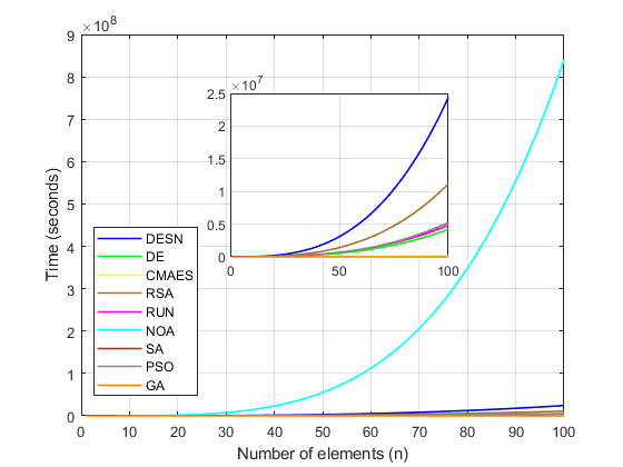
Essentially, the Big O is a mathematical notation utilized in data science to gauge the computational complexity of an algorithm [33]. In simple terms, the Big O analysis establishes four different types of complexity for any algorithm: linear complexity, quadratic complexity, logarithmic complexity, and exponential complexity. The lineal complexity defines those code lines that involve only mathematical operations without being in a loop. The rest of the complexities involve those code lines that belong to a looping process, considering as quadratic complexity those that operate on a linear cumulative iterative process. In contrast, the logarithmic and exponential complexities lie in loops whose iterative process is precisely logarithmic or exponential, respectively. It is worth mentioning that most of the evolutionary computation algorithms have quadratic complexity due to the nature of their programming, while the last two complexities are usually appreciated in machine learning and data mining approaches. Table 6 outlines the Big O notation for the nine examined algorithms. It is evident that NOA exhibited the highest computational complexity among them. As can be noticed, all the algorithms present a quadratic complexity since all of them report an iterative polynomial notation. In simple terms, the exponents represent the number of nested loops, and their respective constants indicate the code line inside said nested loop. As the reader can infer, the higher the number of nested loops and their constants, the higher the complexity of the algorithm.

Table 5 Friedman Rank Test.

Algorithms	Friedman Test	Rank
DESN	1.0833	1
DE	4.8167	5
CMAES	3.7833	3
RSA	7.5333	8
RUN	3.9667	4
NOA	2.7833	2
SA	8.3667	9
PSO	5.5167	6
GA	7.15	7
$p$ -value	3.71E-35

Table 6 Big O notation for the algorithms.

Algorithm	Big O Equation	Notation
DESN	$24n^{3}+37n^{2}+10n+16$	$O(n^{3})$
DE	$4n^{3}+21n^{2}+8n+15$	$O(n^{3})$
CMAES	$15n^{2}+34n+48$	$O(n^{2})$
RSA	$11n^{3}+16n^{2}+10n+14$	$O(n^{3})$
RUN	$4n^{3}+81n^{2}+12n+28$	$O(n^{3})$
NOA	$8n^{4}+40n^{3}+35n^{2}+17n+20$	$O(n^{4})$
SA	$5n^{3}+22n^{2}+n+26$	$O(n^{3})$
PSO	$5n^{3}+17n^{2}+17n+20$	$O(n^{3})$
GA	$5n^{3}+27n^{2}+11n+13$	$O(n^{3})$

Similarly, Figure 5 illustrates the Big O performances of the algorithms, highlighting NOA's significantly higher computational expense compared to others. Conversely, DESN emerged as the most computationally demanding method, followed closely by RSA, while DE and GA demonstrated the least computational overhead due to their algorithmic structures. However, DESN's computational cost is comparable to that of RSA, rendering it a less competitive option.

Figure 5 Big O graphical analysis.

5. Conclusions

This study introduces a novel evolutionary strategy named DESN, which builds upon differential evolution principles. The algorithm features an iterative selection process that dynamically alternates between two popular mutation schemes based on the number of function evaluations. Additionally, it enhances the traditional greedy selection stage of DE by incorporating comparisons not only with the current individual but also with neighboring individuals, representing approximately 25% of the population. These adaptations have notably elevated the algorithm's performance, demonstrating superiority over DE and other approaches across all metric experiments using the CEC-2017 test problems.

The evaluation, which includes Friedman's non-parametric test and Big O analysis, underscores the remarkable competitiveness of the proposed algorithm. However, to further validate its efficacy, DESN necessitates evaluation across diverse benchmark function datasets and testing within high-dimensional problem domains. Furthermore, it is essential to explore its applicability in digital image processing and training machine learning algorithms to ascertain its real-world performance. These avenues, among others, constitute potential directions for future research on DESN. Despite these avenues for exploration, the findings of this study position DESN as a promising evolutionary strategy within the current landscape of optimization techniques.

However, we recognize the challenges associated with this algorithm in certain tasks. We acknowledge its potential in various domains, including multi-objective optimization, in real-world and high-dimensional engineering problems. Consequently, future work will focus on developing this methodology to make it more robust and applicable to different problems, such as implementations with machine learning models.

Data Availability Statement

Data will be made available on request.

Funding

This work was supported without any funding.

Conflicts of Interest

The authors declare no conflicts of interest.

Ethical Approval and Consent to Participate

Not applicable.

References

Storn, R., & Price, K. (1997). Differential evolution--a simple and efficient heuristic for global optimization over continuous spaces. Journal of Global Optimization, 11, 341-359.
[CrossRef] [Google Scholar]
Neri, F., & Tirronen, V. (2019). Recent advances in differential evolution: A survey and experimental analysis. Artificial Intelligence Review, 33, 61–106.
[CrossRef] [Google Scholar]
Sloss, A. N., & Gustafson, S. (2019). 2019 Evolutionary Algorithms Review. Genetic Programming Theory and Practice XVII, 307–344.
[CrossRef] [Google Scholar]
Das, S., & Suganthan, P. N. (2010). Differential evolution: A survey of the state-of-the-art. IEEE Transactions on Evolutionary Computation, 15(1), 4–31.
[CrossRef] [Google Scholar]
Pant, M., Zaheer, H., Garcia-Hernandez, L., & Abraham, A. (2020). Differential Evolution: A review of more than two decades of research. Engineering Applications of Artificial Intelligence, 90, 103479.
[CrossRef] [Google Scholar]
Ahmad, M. F., Isa, N. A. M., Lim, W. H., & Ang, K. M. (2022). Differential evolution with modified initialization scheme using chaotic oppositional based learning strategy. Alexandria Engineering Journal, 61(12), 11835–11858.
[CrossRef] [Google Scholar]
Deng, L., Li, C., Lan, Y., Sun, G., & Shang, C. (2022). Differential evolution with dynamic combination based mutation operator and two-level parameter adaptation strategy. Expert Systems with Applications, 192, 116298.
[CrossRef] [Google Scholar]
Zhang, J., & Sanderson, A. C. (2007, September). JADE: Self-adaptive differential evolution with fast and reliable convergence performance. In 2007 IEEE congress on evolutionary computation (pp. 2251-2258). IEEE.
[CrossRef] [Google Scholar]
Mohamed, A. W. (2015). An improved differential evolution algorithm with triangular mutation for global numerical optimization. Computers and Industrial Engineering, 85, 359–375.
[CrossRef] [Google Scholar]
Prabha, S., & Yadav, R. (2020). Differential evolution with biological-based mutation operator. Engineering Science and Technology, an International Journal, 23(2), 253–263.
[CrossRef] [Google Scholar]
Pant, M., Ali, M., & Singh, V. P. (2008). Differential evolution with parent centric crossover. UKSIM European Symposium on Computer Modeling and Simulation, 2, 141–146.
[CrossRef] [Google Scholar]
Qiu, X., Tan, K. C., & Xu, J. X. (2016). Multiple exponential recombination for differential evolution. IEEE Transactions on Cybernetics, 47(4), 995–1006.
[CrossRef] [Google Scholar]
Zeng, Z., Zhang, M., Chen, T., & Hong, Z. (2021). A new selection operator for differential evolution algorithm. Knowledge-Based Systems, 226, 107150.
[CrossRef] [Google Scholar]
Telikani, A., Tahmassebi, A., Banzhaf, W., & Gandomi, A. H. (2021). Evolutionary machine learning: A survey. ACM Computing Surveys (CSUR), 54(8), 1-35.
[CrossRef] [Google Scholar]
Li, N., Ma, L., Xing, T., Yu, G., Wang, C., Wen, Y., ... & Gao, S. (2023). Automatic design of machine learning via evolutionary computation: A survey. Applied Soft Computing, 143, 110412.
[CrossRef] [Google Scholar]
Zhan, Z. H., Li, J. Y., & Zhang, J. (2022). Evolutionary deep learning: A survey. Neurocomputing, 483, 42-58.
[CrossRef] [Google Scholar]
Gad, A. G. (2022). Particle swarm optimization algorithm and its applications: a systematic review. Archives of computational methods in engineering, 29(5), 2531-2561.
[CrossRef] [Google Scholar]
Katoch, S., Chauhan, S. S., & Kumar, V. (2021). A review on genetic algorithm: past, present, and future. Multimedia tools and applications, 80, 8091-8126.
[CrossRef] [Google Scholar]
Price, K., Storn, R. M., & Lampinen, J. A. (2006). Differential evolution: a practical approach to global optimization. Springer Science & Business Media.
[Google Scholar]
Liang, J. J., Qu, B. Y., Suganthan, P. N., & Hernández-Díaz, A. G. (2013). Problem definitions and evaluation criteria for the CEC 2013 special session on real-parameter optimization. Computational Intelligence Laboratory, Zhengzhou University, Zhengzhou, China and Nanyang Technological University, Singapore, Technical Report, 201212(34), 281–295.
[CrossRef] [Google Scholar]
Brest, J., Greiner, S., Boskovic, B., Mernik, M., & Zumer, V. (2006). Self-adapting control parameters in differential evolution: A comparative study on numerical benchmark problems. IEEE Transactions on Evolutionary Computation, 10(6), 646–657.
[CrossRef] [Google Scholar]
Hansen, N., & Ostermeier, A. (2001). Completely Derandomized Self-Adaptation in Evolution Strategies. Evolutionary Computation, 9(2), 159–195.
[CrossRef] [Google Scholar]
Abualigah, L., Elaziz, M. A., Sumari, P., Geem, Z. W., & Gandomi, A. H. (2022). Reptile Search Algorithm (RSA): A nature-inspired meta-heuristic optimizer. Expert Systems with Applications, 191, 116158.
[CrossRef] [Google Scholar]
Ahmadianfar, I., Heidari, A. A., Gandomi, A. H., Chu, X., & Chen, H. (2021). RUN beyond the metaphor: An efficient optimization algorithm based on Runge Kutta method. Expert Systems with Applications, 181, 115079.
[CrossRef] [Google Scholar]
Basset, M. A., Mohamed, R., Jameel, M., & Abouhawwash, M. (2023). Nutcracker optimizer: A novel nature-inspired metaheuristic algorithm for global optimization and engineering design problems. Knowledge-Based Systems, 262, 110248.
[CrossRef] [Google Scholar]
Bertsimas, D., & Tsitsiklis, J. (1993). Simulated Annealing. Statistical Science, 8(1), 10–15.
[CrossRef] [Google Scholar]
Kennedy, J., & Eberhart, R. (1995). Particle Swarm Optimization. Proceedings of ICNN'95 - International Conference on Neural Networks, 4, 1942–1948.
[CrossRef] [Google Scholar]
Holland, J. H. (1984). Genetic Algorithms and Adaptation. Adaptive Control of Ill-Defined Systems, 16, 317–333.
[CrossRef] [Google Scholar]
Garden, R. W., & Engelbrecht, A. P. (2014). Analysis and Classification of Optimisation Benchmark Functions and Benchmark Suites. IEEE Congress on Evolutionary Computation (CEC), 1641–1649.
[CrossRef] [Google Scholar]
Bagdonavicius, V., Kruopis, J., & Nikulin, M. S. (2013). Nonparametric tests for complete data. John Wiley & Sons.
[Google Scholar]
Friedman, M. (1937). The use of ranks to avoid the assumption of normality implicit in the analysis of variance. Journal of the American Statistical Association, 32(200), 675–701.
[CrossRef] [Google Scholar]
Derrac, J., García, S., Molina, D., & Herrera, F. (2011). A practical tutorial on the use of nonparametric statistical tests as a methodology for comparing evolutionary and swarm intelligence algorithms. Swarm and Evolutionary Computation, 1(1), 3–18.
[CrossRef] [Google Scholar]
Knuth, D. E. (1973). The Art of Computer Programming. Addison-Wesley Publishing Co.
[Google Scholar]
Chen, T., Tang, K., Chen, G., & Yao, X. (2010). Analysis of computational time of simple estimation of distribution algorithms. IEEE Transactions on Evolutionary Computation, 14(1), 1–22.
[CrossRef] [Google Scholar]
Papadimitriou, C. H. (2003). Computational complexity. Encyclopedia of Computer Science, 260–265.
[CrossRef] [Google Scholar]

Cite This Article

APA Style

Reyes-Davila, E., Haro, E. H., Casas-Ordaz, A., Oliva, D., Zapotecas-Martínez, S., & El-Abd, M. (2025). Enhanced Differential Evolution: Multi-Strategy Approach with Neighborhood-Based Selection. IECE Transactions on Swarm and Evolutionary Learning, 1(1), 12–24. https://doi.org/10.62762/TSEL.2025.182681

Article Metrics

Citations:

Google Scholar

0

Crossref

0

Scopus

0

Web of Science

0

Publisher's Note

IECE stays neutral with regard to jurisdictional claims in published maps and institutional affiliations.

Rights and permissions

Institute of Emerging and Computer Engineers (IECE) or its licensor (e.g. a society or other partner) holds exclusive rights to this article under a publishing agreement with the author(s) or other rightsholder(s); author self-archiving of the accepted manuscript version of this article is solely governed by the terms of such publishing agreement and applicable law.

Table of Content